Modeling spectral bands with climlab
Here is a brief introduction to the climlab.BandRCModel process.
This is a model that divides the spectrum into 7 distinct bands: three shortwave and four longwave.
As we will see, the process works much like the familiar climlab.RadiativeConvectiveModel.
About the spectra
The shortwave is divided into three channels:
Channel 0 is the Hartley and Huggins band (extreme UV, 200 - 340 nm, 1% of total flux, strong ozone absorption)
Channel 1 is Chappuis band (450 - 800 nm, 27% of total flux, moderate ozone absorption)
Channel 2 is remaining radiation (72% of total flux, largely in the visible range, no ozone absorption)
The longwave is divided into four bands:
Band 0 is the window region (between 8.5 and 11 \(\mu\)m), 17% of total flux.
Band 1 is the CO2 absorption channel (the band of strong absorption by CO2 around 15 \(\mu\)m), 15% of total flux
Band 2 is a weak water vapor absorption channel, 35% of total flux
Band 3 is a strong water vapor absorption channel, 33% of total flux
The longwave decomposition is not as easily related to specific wavelengths, as in reality there is a lot of overlap between H\(_2\)O and CO\(_2\) absorption features (as well as absorption by other greenhouse gases such as CH\(_4\) and N\(_2\)O that we are not representing).
Example usage of the spectral model
[1]:
%matplotlib inline
import numpy as np
import matplotlib.pyplot as plt
import climlab
from climlab import constants as const
First try a model with all default parameters. Usage is very similar to the familiar RadiativeConvectiveModel.
[2]:
col1 = climlab.BandRCModel()
print(col1)
climlab Process of type <class 'climlab.model.column.BandRCModel'>.
State variables and domain shapes:
  Ts: (1,)
  Tatm: (30,)
The subprocess tree:
Untitled: <class 'climlab.model.column.BandRCModel'>
   LW: <class 'climlab.radiation.nband.FourBandLW'>
   SW: <class 'climlab.radiation.nband.ThreeBandSW'>
   insolation: <class 'climlab.radiation.insolation.FixedInsolation'>
   convective adjustment: <class 'climlab.convection.convadj.ConvectiveAdjustment'>
   H2O: <class 'climlab.radiation.water_vapor.ManabeWaterVapor'>
Check out the list of subprocesses.
We now have a process called H2O, in addition to things we’ve seen before.
This model keeps track of water vapor. We see the specific humidity in the list of state variables:
[3]:
col1.state
[3]:
AttrDict({'Ts': Field([288.]), 'Tatm': Field([200.        , 202.68965517, 205.37931034, 208.06896552,
       210.75862069, 213.44827586, 216.13793103, 218.82758621,
       221.51724138, 224.20689655, 226.89655172, 229.5862069 ,
       232.27586207, 234.96551724, 237.65517241, 240.34482759,
       243.03448276, 245.72413793, 248.4137931 , 251.10344828,
       253.79310345, 256.48275862, 259.17241379, 261.86206897,
       264.55172414, 267.24137931, 269.93103448, 272.62068966,
       275.31034483, 278.        ])})
The water vapor field is initialized to zero. The H2O process will set the specific humidity field at every timestep to a specified profile. More on that below. For now, let’s compute a radiative equilibrium state.
[4]:
col1.integrate_years(2)
Integrating for 730 steps, 730.4844 days, or 2 years.
Total elapsed time is 1.9986737567564754 years.
[5]:
# Check for energy balance
col1.ASR - col1.OLR
[5]:
Field([-0.00148377])
[6]:
fig = plt.figure()
ax = fig.add_subplot(111)
ax.plot( col1.Tatm, col1.lev, 'c-', label='default' )
ax.plot( col1.Ts, climlab.constants.ps, 'co', markersize=16 )
ax.invert_yaxis()
ax.set_xlabel('Temperature (K)', fontsize=16)
ax.set_ylabel('Pressure (hPa)', fontsize=16 )
ax.set_title('Temperature profiles', fontsize = 18)
ax.grid()
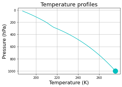
By default this model has convective adjustment. We can set the adjusted lapse rate by passing a parameter when we create the model.
The model currently has no ozone (so there is no stratosphere). Not very realistic!
More reasonable-looking troposphere, but still no stratosphere.
About the radiatively active gases
The Band model is aware of three different absorbing gases: O3 (ozone), CO2, and H2O (water vapor). The abundances of these gases are stored in a dictionary of arrays as follows:
[7]:
col1.absorber_vmr
[7]:
{'CO2': Field([0.00038, 0.00038, 0.00038, 0.00038, 0.00038, 0.00038, 0.00038,
        0.00038, 0.00038, 0.00038, 0.00038, 0.00038, 0.00038, 0.00038,
        0.00038, 0.00038, 0.00038, 0.00038, 0.00038, 0.00038, 0.00038,
        0.00038, 0.00038, 0.00038, 0.00038, 0.00038, 0.00038, 0.00038,
        0.00038, 0.00038]),
 'O3': Field([0., 0., 0., 0., 0., 0., 0., 0., 0., 0., 0., 0., 0., 0., 0., 0., 0.,
        0., 0., 0., 0., 0., 0., 0., 0., 0., 0., 0., 0., 0.]),
 'H2O': Field([5.00000000e-06, 5.00000000e-06, 5.00000000e-06, 5.00000000e-06,
        5.00000000e-06, 5.00000000e-06, 6.38590233e-06, 9.08848690e-06,
        1.33273826e-05, 2.34389689e-05, 3.84220914e-05, 5.95564299e-05,
        8.82144990e-05, 1.25843839e-04, 1.73951159e-04, 2.34088411e-04,
        3.07840683e-04, 3.96815735e-04, 5.02635028e-04, 6.26926041e-04,
        7.71315753e-04, 9.37425100e-04, 1.12686431e-03, 1.34122899e-03,
        1.58209684e-03, 1.85102493e-03, 2.14954752e-03, 2.47917415e-03,
        2.84138824e-03, 3.23764591e-03])}
Ozone and CO2 are both specified in the model. The default, as you see above, is zero ozone, and constant (well-mixed) CO2 at a volume mixing ratio of 3.8E-4 or 380 ppm.
Water vapor is handled differently: it is determined by the model at each timestep. We make the following assumptions, following a classic paper on radiative-convective equilibrium by Manabe and Wetherald (J. Atmos. Sci. 1967):
the relative humidity just above the surface is fixed at 77% (can be changed of course… see the parameter
col1.relative_humiditywater vapor drops off linearly with pressure
there is a small specified amount of water vapor in the stratosphere.
Putting in some ozone
[8]:
#  Put in some ozone
import xarray as xr

ozonepath = "http://thredds.atmos.albany.edu:8080/thredds/dodsC/CLIMLAB/ozone/apeozone_cam3_5_54.nc"
ozone = xr.open_dataset(ozonepath)
ozone
[8]:
<xarray.Dataset>
Dimensions:    (lat: 64, lev: 59, lon: 128, time: 12)
Coordinates:
  * lev        (lev) float64 0.2842 0.3253 0.3719 ... 849.5 959.0 1.004e+03
  * lon        (lon) float64 0.0 2.812 5.625 8.438 ... 348.8 351.6 354.4 357.2
  * lat        (lat) float64 -87.86 -85.1 -82.31 -79.53 ... 82.31 85.1 87.86
  * time       (time) float64 4.382e+04 4.384e+04 ... 4.412e+04 4.415e+04
Data variables:
    P0         float64 1.004e+05
    date       (time) int32 19900116 19900214 19900316 ... 19901115 19901216
    datesec    (time) int32 0 0 0 0 0 0 0 0 0 0 0 0
    OZONE_old  (time, lat, lev, lon) float64 ...
    OZONE      (time, lev, lat, lon) float64 ...
Attributes:
    Conventions:                     NCAR-CSM
    Source:                          AMIP II (symmetric for APE project)
    Written_By:                      olson
    Date_Written:                    August 22 2003
    Host:                            zen
    Command:                         ncgen
    history:                         Wed Jul 30 08:35:58 2008: ncrename -v OZ...
DODS_EXTRA.Unlimited_Dimension: time- lat: 64
- lev: 59
- lon: 128
- time: 12
- lev(lev)float640.2842 0.3253 ... 959.0 1.004e+03
- long_name :
- hybrid level at layer midpoints (1000*(A+B))
- units :
- hybrid_sigma_pressure
- positive :
- down
array([2.84191e-01, 3.25350e-01, 3.71936e-01, 4.24615e-01, 4.84153e-01, 5.51432e-01, 6.27490e-01, 7.13542e-01, 8.11039e-01, 9.21699e-01, 1.04757e+00, 1.19108e+00, 1.35511e+00, 1.54305e+00, 1.75891e+00, 2.00739e+00, 2.29403e+00, 2.62529e+00, 3.00884e+00, 3.45369e+00, 3.97050e+00, 4.57190e+00, 5.27278e+00, 6.09073e+00, 7.04636e+00, 8.16371e+00, 9.47075e+00, 1.10000e+01, 1.27894e+01, 1.48832e+01, 1.73342e+01, 2.02039e+01, 2.35659e+01, 2.75066e+01, 3.21283e+01, 3.75509e+01, 4.39150e+01, 5.13840e+01, 6.01483e+01, 7.04289e+01, 8.24830e+01, 9.66096e+01, 1.13155e+02, 1.32514e+02, 1.55122e+02, 1.81445e+02, 2.11947e+02, 2.47079e+02, 2.87273e+02, 3.32956e+02, 3.84573e+02, 4.42610e+02, 5.07601e+02, 5.80132e+02, 6.60837e+02, 7.50393e+02, 8.49521e+02, 9.58981e+02, 1.00369e+03]) - lon(lon)float640.0 2.812 5.625 ... 354.4 357.2
- long_name :
- longitude
- units :
- degrees_east
array([ 0. , 2.8125, 5.625 , 8.4375, 11.25 , 14.0625, 16.875 , 19.6875, 22.5 , 25.3125, 28.125 , 30.9375, 33.75 , 36.5625, 39.375 , 42.1875, 45. , 47.8125, 50.625 , 53.4375, 56.25 , 59.0625, 61.875 , 64.6875, 67.5 , 70.3125, 73.125 , 75.9375, 78.75 , 81.5625, 84.375 , 87.1875, 90. , 92.8125, 95.625 , 98.4375, 101.25 , 104.0625, 106.875 , 109.6875, 112.5 , 115.3125, 118.125 , 120.9375, 123.75 , 126.5625, 129.375 , 132.1875, 135. , 137.8125, 140.625 , 143.4375, 146.25 , 149.0625, 151.875 , 154.6875, 157.5 , 160.3125, 163.125 , 165.9375, 168.75 , 171.5625, 174.375 , 177.1875, 180. , 182.8125, 185.625 , 188.4375, 191.25 , 194.0625, 196.875 , 199.6875, 202.5 , 205.3125, 208.125 , 210.9375, 213.75 , 216.5625, 219.375 , 222.1875, 225. , 227.8125, 230.625 , 233.4375, 236.25 , 239.0625, 241.875 , 244.6875, 247.5 , 250.3125, 253.125 , 255.9375, 258.75 , 261.5625, 264.375 , 267.1875, 270. , 272.8125, 275.625 , 278.4375, 281.25 , 284.0625, 286.875 , 289.6875, 292.5 , 295.3125, 298.125 , 300.9375, 303.75 , 306.5625, 309.375 , 312.1875, 315. , 317.8125, 320.625 , 323.4375, 326.25 , 329.0625, 331.875 , 334.6875, 337.5 , 340.3125, 343.125 , 345.9375, 348.75 , 351.5625, 354.375 , 357.1875]) - lat(lat)float64-87.86 -85.1 -82.31 ... 85.1 87.86
- long_name :
- latitude
- units :
- degrees_north
array([-87.8638, -85.0965, -82.3129, -79.5256, -76.7369, -73.9475, -71.1577, -68.3678, -65.5776, -62.7873, -59.997 , -57.2066, -54.4162, -51.6257, -48.8352, -46.0447, -43.2542, -40.4636, -37.6731, -34.8825, -32.0919, -29.3014, -26.5108, -23.7202, -20.9296, -18.139 , -15.3484, -12.5578, -9.7671, -6.9765, -4.1859, -1.3953, 1.3953, 4.1859, 6.9765, 9.7671, 12.5578, 15.3484, 18.139 , 20.9296, 23.7202, 26.5108, 29.3014, 32.0919, 34.8825, 37.6731, 40.4636, 43.2542, 46.0447, 48.8352, 51.6257, 54.4162, 57.2066, 59.997 , 62.7873, 65.5776, 68.3678, 71.1577, 73.9475, 76.7369, 79.5256, 82.3129, 85.0965, 87.8638]) - time(time)float644.382e+04 4.384e+04 ... 4.415e+04
- long_name :
- time
- units :
- day number (Jan 1 = 1)
- calendar :
- 365_days
array([43816., 43844., 43875., 43905., 43936., 43966., 43997., 44028., 44058.,
       44089., 44119., 44150.])
- P0()float64...
- long_name :
- reference pressure
- units :
- Pa
array(100369.)
- date(time)int32...
- long_name :
- current date as 8 digit integer (YYYYMMDD)
array([19900116, 19900214, 19900316, 19900415, 19900516, 19900615, 19900716, 19900816, 19900915, 19901016, 19901115, 19901216], dtype=int32) - datesec(time)int32...
- long_name :
- seconds of current date
- units :
- s
array([0, 0, 0, 0, 0, 0, 0, 0, 0, 0, 0, 0], dtype=int32)
- OZONE_old(time, lat, lev, lon)float64...
- long_name :
- OZONE
- units :
- FRACTION
[5799936 values with dtype=float64]
- OZONE(time, lev, lat, lon)float64...
- long_name :
- OZONE
- units :
- FRACTION
[5799936 values with dtype=float64]
- Conventions :
- NCAR-CSM
- Source :
- AMIP II (symmetric for APE project)
- Written_By :
- olson
- Date_Written :
- August 22 2003
- Host :
- zen
- Command :
- ncgen
- history :
- Wed Jul 30 08:35:58 2008: ncrename -v OZONE,OZONE_old apeozone_cam3_5_54.nc
- DODS_EXTRA.Unlimited_Dimension :
- time
[9]:
#  Dimensions of the ozone file
lat = ozone.lat
lon = ozone.lon
lev = ozone.lev
[10]:
# Taking annual, zonal, and global averages of the ozone data
O3_zon = ozone.OZONE.mean(dim=("time","lon"))

weight_ozone = np.cos(np.deg2rad(ozone.lat)) / np.cos(np.deg2rad(ozone.lat)).mean(dim='lat')
O3_global = (O3_zon * weight_ozone).mean(dim='lat')
[11]:
fig = plt.figure()
ax = fig.add_subplot(111)
ax.plot( O3_global*1E6, lev)
ax.invert_yaxis()
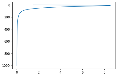
We are going to create another instance of the model, this time using the same vertical coordinates as the ozone data.
[12]:
#  Create the column with appropriate vertical coordinate, surface albedo and convective adjustment
col2 = climlab.BandRCModel(lev=lev)
print(col2)
climlab Process of type <class 'climlab.model.column.BandRCModel'>.
State variables and domain shapes:
  Ts: (1,)
  Tatm: (59,)
The subprocess tree:
Untitled: <class 'climlab.model.column.BandRCModel'>
   LW: <class 'climlab.radiation.nband.FourBandLW'>
   SW: <class 'climlab.radiation.nband.ThreeBandSW'>
   insolation: <class 'climlab.radiation.insolation.FixedInsolation'>
   convective adjustment: <class 'climlab.convection.convadj.ConvectiveAdjustment'>
   H2O: <class 'climlab.radiation.water_vapor.ManabeWaterVapor'>
[13]:
#  Set the ozone mixing ratio
col2.absorber_vmr['O3'] = O3_global.values
[14]:
#  Run the model out to equilibrium!
col2.integrate_years(2.)
Integrating for 730 steps, 730.4844 days, or 2.0 years.
Total elapsed time is 1.9986737567564754 years.
[15]:
fig = plt.figure()
ax = fig.add_subplot(111)
ax.plot( col1.Tatm, np.log(col1.lev/1000), 'c-', label='RCE' )
ax.plot( col1.Ts, 0, 'co', markersize=16 )
ax.plot(col2.Tatm, np.log(col2.lev/1000), 'r-', label='RCE O3' )
ax.plot(col2.Ts, 0, 'ro', markersize=16 )
ax.invert_yaxis()
ax.set_xlabel('Temperature (K)', fontsize=16)
ax.set_ylabel('log(Pressure)', fontsize=16 )
ax.set_title('Temperature profiles', fontsize = 18)
ax.grid()
ax.legend()
[15]:
<matplotlib.legend.Legend at 0x169c510d0>
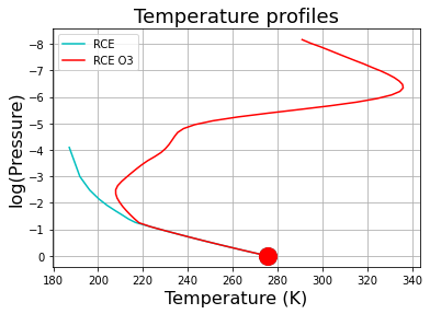
Once we include ozone we get a well-defined stratosphere. We can also a slight cooling effect in the troposphere.
Things to consider / try:
Here we used the global annual mean Q = 341.3 W m\(^{-2}\). We might want to consider latitudinal or seasonal variations in Q.
We also used the global annual mean ozone profile! Ozone varies tremendously in latitude and by season. That information is all contained in the ozone data file we opened above. We might explore the effects of those variations.
We can calculate climate sensitivity in this model by doubling the CO2 concentration and re-running out to the new equilibrium. Does the amount of ozone affect the climate sensitivity? (example below)
An important shortcoming of the model: there are no clouds! (that would be the next step in the hierarchy of column models)
Clouds would act both in the shortwave (increasing the albedo, cooling the climate) and in the longwave (greenhouse effect, warming the climate). Which effect is stronger depends on the vertical structure of the clouds (high or low clouds) and their optical properties (e.g. thin cirrus clouds are nearly transparent to solar radiation but are good longwave absorbers).
[16]:
col3 = climlab.process_like(col2)
print(col3)
climlab Process of type <class 'climlab.model.column.BandRCModel'>.
State variables and domain shapes:
  Ts: (1,)
  Tatm: (59,)
The subprocess tree:
Untitled: <class 'climlab.model.column.BandRCModel'>
   LW: <class 'climlab.radiation.nband.FourBandLW'>
   SW: <class 'climlab.radiation.nband.ThreeBandSW'>
   insolation: <class 'climlab.radiation.insolation.FixedInsolation'>
   convective adjustment: <class 'climlab.convection.convadj.ConvectiveAdjustment'>
   H2O: <class 'climlab.radiation.water_vapor.ManabeWaterVapor'>
[17]:
# Let's double CO2.
col3.absorber_vmr['CO2'] *= 2.
[18]:
col3.compute_diagnostics()
print('The radiative forcing for doubling CO2 is %f W/m2.' % (col2.OLR - col3.OLR))
The radiative forcing for doubling CO2 is 1.310158 W/m2.
[19]:
col3.integrate_years(3)
Integrating for 1095 steps, 1095.7266 days, or 3 years.
Total elapsed time is 4.996684391891189 years.
[20]:
col3.ASR - col3.OLR
[20]:
Field([3.98517386e-07])
[21]:
print('The Equilibrium Climate Sensitivity is %f K.' % (col3.Ts - col2.Ts))
The Equilibrium Climate Sensitivity is 2.758433 K.
[22]:
col4 = climlab.process_like(col1)
print(col4)
climlab Process of type <class 'climlab.model.column.BandRCModel'>.
State variables and domain shapes:
  Ts: (1,)
  Tatm: (30,)
The subprocess tree:
Untitled: <class 'climlab.model.column.BandRCModel'>
   LW: <class 'climlab.radiation.nband.FourBandLW'>
   SW: <class 'climlab.radiation.nband.ThreeBandSW'>
   insolation: <class 'climlab.radiation.insolation.FixedInsolation'>
   convective adjustment: <class 'climlab.convection.convadj.ConvectiveAdjustment'>
   H2O: <class 'climlab.radiation.water_vapor.ManabeWaterVapor'>
[23]:
col4.absorber_vmr
[23]:
{'CO2': Field([0.00038, 0.00038, 0.00038, 0.00038, 0.00038, 0.00038, 0.00038,
        0.00038, 0.00038, 0.00038, 0.00038, 0.00038, 0.00038, 0.00038,
        0.00038, 0.00038, 0.00038, 0.00038, 0.00038, 0.00038, 0.00038,
        0.00038, 0.00038, 0.00038, 0.00038, 0.00038, 0.00038, 0.00038,
        0.00038, 0.00038]),
 'O3': Field([0., 0., 0., 0., 0., 0., 0., 0., 0., 0., 0., 0., 0., 0., 0., 0., 0.,
        0., 0., 0., 0., 0., 0., 0., 0., 0., 0., 0., 0., 0.]),
 'H2O': Field([5.00000000e-06, 5.00000000e-06, 5.00000000e-06, 5.00000000e-06,
        5.00000000e-06, 5.00000000e-06, 6.38590233e-06, 9.08848690e-06,
        1.33273826e-05, 2.34389689e-05, 3.84220914e-05, 5.95564299e-05,
        8.82144990e-05, 1.25843839e-04, 1.73951159e-04, 2.34088411e-04,
        3.07840683e-04, 3.96815735e-04, 5.02635028e-04, 6.26926041e-04,
        7.71315753e-04, 9.37425100e-04, 1.12686431e-03, 1.34122899e-03,
        1.58209684e-03, 1.85102493e-03, 2.14954752e-03, 2.47917415e-03,
        2.84138824e-03, 3.23764591e-03])}
[24]:
col4.absorber_vmr['CO2'] *= 2.
col4.compute_diagnostics()
print('The radiative forcing for doubling CO2 is %f W/m2.' % (col1.OLR - col4.OLR))
The radiative forcing for doubling CO2 is 4.421081 W/m2.
[25]:
col4.integrate_years(3.)
col4.ASR - col4.OLR
Integrating for 1095 steps, 1095.7266 days, or 3.0 years.
Total elapsed time is 4.996684391891189 years.
[25]:
Field([-5.25654883e-07])
[26]:
print('The Equilibrium Climate Sensitivity is %f K.' % (col4.Ts - col1.Ts))
The Equilibrium Climate Sensitivity is 3.180993 K.
Interesting that the model is MORE sensitive when ozone is set to zero.
[ ]: