Radiative-Convective Equilibrium with CAM3 scheme¶

[1]:

%matplotlib inline
import numpy as np
import matplotlib.pyplot as plt
import climlab
from climlab import constants as const

Here is how to set a simple RCE in `climlab`¶

By initializing each component with the same state object, the components are already effectively coupled. They all act to modify the same state object.

No extra coupling code is necessary.

[2]:

# initial state (temperatures)
state = climlab.column_state(num_lev=20, num_lat=1, water_depth=5.)

[3]:

## Create individual physical process models:
#  fixed relative humidity
h2o = climlab.radiation.ManabeWaterVapor(name='H2O', state=state)
#  Hard convective adjustment
convadj = climlab.convection.ConvectiveAdjustment(name='Convective Adjustment',
                                                  state=state,
                                                  adj_lapse_rate=6.5)
# CAM3 radiation with default parameters and interactive water vapor
rad = climlab.radiation.CAM3(name='Radiation',
                             state=state,
                             specific_humidity=h2o.q)

rce = climlab.couple([rad,convadj,h2o], name='RCM')

[4]:

print(rce)

climlab Process of type <class 'climlab.process.time_dependent_process.TimeDependentProcess'>.
State variables and domain shapes:
  Ts: (1,)
  Tatm: (20,)
The subprocess tree:
RCM: <class 'climlab.process.time_dependent_process.TimeDependentProcess'>
   Radiation: <class 'climlab.radiation.cam3.cam3.CAM3'>
   Convective Adjustment: <class 'climlab.convection.convadj.ConvectiveAdjustment'>
   H2O: <class 'climlab.radiation.water_vapor.ManabeWaterVapor'>

[5]:

#  Current state
rce.state

[5]:

AttrDict({'Ts': Field([288.]), 'Tatm': Field([200.        , 204.10526316, 208.21052632, 212.31578947,
       216.42105263, 220.52631579, 224.63157895, 228.73684211,
       232.84210526, 236.94736842, 241.05263158, 245.15789474,
       249.26315789, 253.36842105, 257.47368421, 261.57894737,
       265.68421053, 269.78947368, 273.89473684, 278.        ])})

[6]:

#  Integrate the model forward
rce.integrate_years(5)

Integrating for 1826 steps, 1826.2110000000002 days, or 5 years.
Total elapsed time is 4.999422301147019 years.

[7]:

#  Current state
rce.state

[7]:

AttrDict({'Ts': Field([276.77058287]), 'Tatm': Field([233.26150428, 215.95044945, 210.60589023, 211.45113437,
       212.04321205, 216.46759988, 223.46187556, 229.6327028 ,
       235.16956012, 240.2017945 , 244.8218937 , 249.09842749,
       253.08373297, 256.81872305, 260.33602553, 263.66210602,
       266.81874721, 269.82410613, 272.69348696, 275.43991673])})

[8]:

#  Current specific humidity
rce.q

[8]:

Field([1.87420483e-05, 9.64556905e-06, 5.58553481e-06, 6.57792987e-06,
       7.30688198e-06, 1.30016777e-05, 3.02115363e-05, 6.04582768e-05,
       1.08656640e-04, 1.80140927e-04, 2.80533313e-04, 4.15636693e-04,
       5.91349145e-04, 8.13596531e-04, 1.08827995e-03, 1.42123518e-03,
       1.81820176e-03, 2.28479967e-03, 2.82651219e-03, 3.44867359e-03])

[9]:

#  Here is the dictionary of input fields for the CAM3 radiation module
rce.subprocess.Radiation.input

[9]:

{'specific_humidity': Field([1.87420483e-05, 9.64556905e-06, 5.58553481e-06, 6.57792987e-06,
        7.30688198e-06, 1.30016777e-05, 3.02115363e-05, 6.04582768e-05,
        1.08656640e-04, 1.80140927e-04, 2.80533313e-04, 4.15636693e-04,
        5.91349145e-04, 8.13596531e-04, 1.08827995e-03, 1.42123518e-03,
        1.81820176e-03, 2.28479967e-03, 2.82651219e-03, 3.44867359e-03]),
 'absorber_vmr': {'CO2': 0.000348,
  'CH4': 1.65e-06,
  'N2O': 3.06e-07,
  'O2': 0.21,
  'CFC11': 0.0,
  'CFC12': 0.0,
  'CFC22': 0.0,
  'CCL4': 0.0,
  'O3': array([5.38853507e-06, 9.86362297e-07, 3.46334801e-07, 1.90806332e-07,
         1.19700066e-07, 7.69083554e-08, 5.97316411e-08, 5.27011190e-08,
         4.80406196e-08, 4.44967931e-08, 4.18202246e-08, 3.99595858e-08,
         3.83838549e-08, 3.66179869e-08, 3.42885526e-08, 3.18505117e-08,
         2.93003951e-08, 2.69906527e-08, 2.49122466e-08, 2.28798533e-08])},
 'cldfrac': 0.0,
 'clwp': 0.0,
 'ciwp': 0.0,
 'r_liq': 0.0,
 'r_ice': 0.0,
 'emissivity': 1.0,
 'S0': 1365.2,
 'insolation': 341.3,
 'coszen': 0.25,
 'eccentricity_factor': 1.0,
 'aldif': 0.3,
 'aldir': 0.3,
 'asdif': 0.3,
 'asdir': 0.3}

Latitudinally, seasonally varying RCE¶

[10]:

# initial state (temperatures)
state2 = climlab.column_state(num_lev=20, num_lat=30, water_depth=10.)

[11]:

#  Create a parent process
rcelat = climlab.TimeDependentProcess(state=state2)
## Create individual physical process models:
#  seasonal insolation
insol = climlab.radiation.DailyInsolation(name='Insolation',
                                          domains=state2['Ts'].domain)
#  fixed relative humidity
h2o = climlab.radiation.ManabeWaterVapor(name='H2O',
                                         state=state2)
#  Hard convective adjustment
convadj = climlab.convection.ConvectiveAdjustment(name='Convective Adjustment',
                                                  state=state2,
                                                  adj_lapse_rate=6.5)
# CAM3 radiation with interactive insolation and interactive water vapor
rad = climlab.radiation.CAM3(name='Radiation',
                             state=state2,
                             specific_humidity=h2o.q,
                             S0 = insol.S0,
                             insolation=insol.insolation,
                             coszen=insol.coszen)

rcelat = climlab.couple([insol,rad,convadj,h2o], name='Seasonal RCE')

print(rcelat)

climlab Process of type <class 'climlab.process.time_dependent_process.TimeDependentProcess'>.
State variables and domain shapes:
  Ts: (30, 1)
  Tatm: (30, 20)
The subprocess tree:
Seasonal RCE: <class 'climlab.process.time_dependent_process.TimeDependentProcess'>
   Insolation: <class 'climlab.radiation.insolation.DailyInsolation'>
   Radiation: <class 'climlab.radiation.cam3.cam3.CAM3'>
   Convective Adjustment: <class 'climlab.convection.convadj.ConvectiveAdjustment'>
   H2O: <class 'climlab.radiation.water_vapor.ManabeWaterVapor'>

[12]:

rcelat.integrate_years(5)

Integrating for 1826 steps, 1826.2110000000002 days, or 5 years.
Total elapsed time is 4.999422301147019 years.

[13]:

rcelat.integrate_years(1)

Integrating for 365 steps, 365.2422 days, or 1 years.
Total elapsed time is 5.9987591795252575 years.

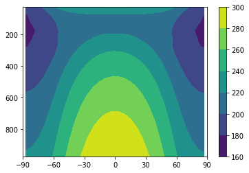
[14]:

def plot_temp_section(model, timeave=True):
    fig = plt.figure()
    ax = fig.add_subplot(111)
    if timeave:
        field = model.timeave['Tatm'].transpose()
    else:
        field = model.Tatm.transpose()
    cax = ax.contourf(model.lat, model.lev, field)
    ax.invert_yaxis()
    ax.set_xlim(-90,90)
    ax.set_xticks([-90, -60, -30, 0, 30, 60, 90])
    fig.colorbar(cax)

[15]:

plot_temp_section(rcelat)

../_images/courseware_RCE_with_CAM3_radiation_17_0.png

Same thing, but also including meridional temperature diffusion¶

[16]:

#  Create and exact clone of the previous model
diffmodel = climlab.process_like(rcelat)
diffmodel.name = 'Seasonal RCE with heat transport'

[17]:

# thermal diffusivity in W/m**2/degC
D = 0.05
# meridional diffusivity in m**2/s
K = D / diffmodel.Tatm.domain.heat_capacity[0] * const.a**2
print(K)

3964424.9422310763

[18]:

d = climlab.dynamics.MeridionalDiffusion(K=K, state={'Tatm': diffmodel.Tatm}, **diffmodel.param)

[19]:

diffmodel.add_subprocess('Meridional Diffusion', d)
print(diffmodel)

climlab Process of type <class 'climlab.process.time_dependent_process.TimeDependentProcess'>.
State variables and domain shapes:
  Ts: (30, 1)
  Tatm: (30, 20)
The subprocess tree:
Seasonal RCE with heat transport: <class 'climlab.process.time_dependent_process.TimeDependentProcess'>
   Insolation: <class 'climlab.radiation.insolation.DailyInsolation'>
   Radiation: <class 'climlab.radiation.cam3.cam3.CAM3'>
   Convective Adjustment: <class 'climlab.convection.convadj.ConvectiveAdjustment'>
   H2O: <class 'climlab.radiation.water_vapor.ManabeWaterVapor'>
   Meridional Diffusion: <class 'climlab.dynamics.meridional_advection_diffusion.MeridionalDiffusion'>

[20]:

diffmodel.integrate_years(5)

Integrating for 1826 steps, 1826.2110000000002 days, or 5 years.
Total elapsed time is 10.998181480672276 years.

[21]:

diffmodel.integrate_years(1)

Integrating for 365 steps, 365.2422 days, or 1 years.
Total elapsed time is 11.997518359050515 years.

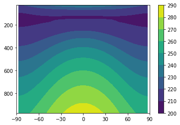
[22]:

plot_temp_section(rcelat)
plot_temp_section(diffmodel)

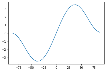
../_images/courseware_RCE_with_CAM3_radiation_25_0.png

../_images/courseware_RCE_with_CAM3_radiation_25_1.png

[23]:

def inferred_heat_transport( energy_in, lat_deg ):
    '''Returns the inferred heat transport (in PW) by integrating the net energy imbalance from pole to pole.'''
    from scipy import integrate
    from climlab import constants as const
    lat_rad = np.deg2rad( lat_deg )
    return ( 1E-15 * 2 * np.math.pi * const.a**2 * integrate.cumtrapz( np.cos(lat_rad)*energy_in,
            x=lat_rad, initial=0. ) )

[24]:

#  Plot the northward heat transport in this model
Rtoa = np.squeeze(diffmodel.timeave['ASR'] - diffmodel.timeave['OLR'])
plt.plot(diffmodel.lat, inferred_heat_transport(Rtoa, diffmodel.lat))

[24]:

[<matplotlib.lines.Line2D at 0x16035fee0>]

../_images/courseware_RCE_with_CAM3_radiation_27_1.png

If you want explicit surface fluxes…¶

All the models above use a convective adjustment that simultaneously adjustments Tatm and Ts to the prescribed lapse rate.

We can instead limit the convective adjustment to just the atmosphere. To do this, we just have to change the state variable dictionary in the convective adjustment process.

Then we can invoke process models for sensible and latent heat fluxes that use simple bulk formulae. Tunable parameters for these include drag coefficient and surface wind speed.

[25]:

diffmodel2 = climlab.process_like(diffmodel)
diffmodel2.name = "Seasonal RCE with surface fluxes and heat transport"

#  Hard convective adjustment -- ATMOSPHERE ONLY
convadj2 = climlab.convection.ConvectiveAdjustment(state={'Tatm':diffmodel2.Tatm}, adj_lapse_rate=6.5)
diffmodel2.add_subprocess('ConvectiveAdjustment', convadj2)

print(diffmodel2)

climlab Process of type <class 'climlab.process.time_dependent_process.TimeDependentProcess'>.
State variables and domain shapes:
  Ts: (30, 1)
  Tatm: (30, 20)
The subprocess tree:
Seasonal RCE with surface fluxes and heat transport: <class 'climlab.process.time_dependent_process.TimeDependentProcess'>
   Insolation: <class 'climlab.radiation.insolation.DailyInsolation'>
   Radiation: <class 'climlab.radiation.cam3.cam3.CAM3'>
   Convective Adjustment: <class 'climlab.convection.convadj.ConvectiveAdjustment'>
   H2O: <class 'climlab.radiation.water_vapor.ManabeWaterVapor'>
   Meridional Diffusion: <class 'climlab.dynamics.meridional_advection_diffusion.MeridionalDiffusion'>
   ConvectiveAdjustment: <class 'climlab.convection.convadj.ConvectiveAdjustment'>

[26]:

#  Now add surface flux processes
#  Add surface heat fluxes

shf = climlab.surface.SensibleHeatFlux(state=diffmodel2.state, Cd=0.5E-3)
lhf = climlab.surface.LatentHeatFlux(state=diffmodel2.state, Cd=0.5E-3)
#  set the water vapor input field for LHF process
lhf.q = diffmodel2.subprocess['H2O'].q
diffmodel2.add_subprocess('SHF', shf)
diffmodel2.add_subprocess('LHF', lhf)

print(diffmodel2)

climlab Process of type <class 'climlab.process.time_dependent_process.TimeDependentProcess'>.
State variables and domain shapes:
  Ts: (30, 1)
  Tatm: (30, 20)
The subprocess tree:
Seasonal RCE with surface fluxes and heat transport: <class 'climlab.process.time_dependent_process.TimeDependentProcess'>
   Insolation: <class 'climlab.radiation.insolation.DailyInsolation'>
   Radiation: <class 'climlab.radiation.cam3.cam3.CAM3'>
   Convective Adjustment: <class 'climlab.convection.convadj.ConvectiveAdjustment'>
   H2O: <class 'climlab.radiation.water_vapor.ManabeWaterVapor'>
   Meridional Diffusion: <class 'climlab.dynamics.meridional_advection_diffusion.MeridionalDiffusion'>
   ConvectiveAdjustment: <class 'climlab.convection.convadj.ConvectiveAdjustment'>
   SHF: <class 'climlab.surface.turbulent.SensibleHeatFlux'>
   LHF: <class 'climlab.surface.turbulent.LatentHeatFlux'>

[27]:

diffmodel2.integrate_years(5)

Integrating for 1826 steps, 1826.2110000000002 days, or 5 years.
Total elapsed time is 16.996940660197534 years.

[28]:

diffmodel2.integrate_years(1)

Integrating for 365 steps, 365.2422 days, or 1 years.
Total elapsed time is 17.99627753857577 years.

[29]:

plot_temp_section(rcelat)
plot_temp_section(diffmodel2)

../_images/courseware_RCE_with_CAM3_radiation_33_0.png

../_images/courseware_RCE_with_CAM3_radiation_33_1.png

[30]:

#  Plot the northward heat transport in this model
Rtoa = np.squeeze(diffmodel2.timeave['ASR'] - diffmodel2.timeave['OLR'])
plt.plot(diffmodel2.lat, inferred_heat_transport(Rtoa, diffmodel2.lat))

[30]:

[<matplotlib.lines.Line2D at 0x16044e310>]

../_images/courseware_RCE_with_CAM3_radiation_34_1.png

[ ]: