Preconfigured Energy Balance Models
In this document the basic use of climlab’s preconfigured EBM class is shown.
Contents are how to
setup an EBM model
show and access subprocesses
integrate the model
access and plot various model variables
calculate the global mean of the temperature
[1]:
%matplotlib inline
import numpy as np
import matplotlib.pyplot as plt
import climlab
from climlab import constants as const
Model Creation
The regular path for the EBM class is climlab.model.ebm.EBM but it can also be accessed through climlab.EBM
An EBM model instance is created through
[2]:
# model creation
ebm_model = climlab.EBM(name='My EBM')
By default many parameters are set during initialization:
num_lat=90, S0=const.S0, A=210., B=2., D=0.55, water_depth=10., Tf=-10, a0=0.3, a2=0.078, ai=0.62, timestep=const.seconds_per_year/90., T0=12., T2=-40
For further details see the climlab documentation.
Many of the input parameters are stored in the following dictionary:
[3]:
# print model parameters
ebm_model.param
[3]:
{'timestep': 350632.51200000005,
 'S0': 1365.2,
 's2': -0.48,
 'A': 210.0,
 'B': 2.0,
 'D': 0.555,
 'Tf': -10.0,
 'water_depth': 10.0,
 'a0': 0.3,
 'a2': 0.078,
 'ai': 0.62}
The model consists of one state variable (surface temperature) and a couple of defined subprocesses.
[4]:
# print model states and suprocesses
print(ebm_model)
climlab Process of type <class 'climlab.model.ebm.EBM'>.
State variables and domain shapes:
  Ts: (90, 1)
The subprocess tree:
My EBM: <class 'climlab.model.ebm.EBM'>
   LW: <class 'climlab.radiation.aplusbt.AplusBT'>
   insolation: <class 'climlab.radiation.insolation.P2Insolation'>
   albedo: <class 'climlab.surface.albedo.StepFunctionAlbedo'>
      iceline: <class 'climlab.surface.albedo.Iceline'>
      warm_albedo: <class 'climlab.surface.albedo.P2Albedo'>
      cold_albedo: <class 'climlab.surface.albedo.ConstantAlbedo'>
   SW: <class 'climlab.radiation.absorbed_shorwave.SimpleAbsorbedShortwave'>
   diffusion: <class 'climlab.dynamics.meridional_heat_diffusion.MeridionalHeatDiffusion'>
Model subprocesses
The subprocesses are stored in a dictionary and can be accessed through
[5]:
# access model subprocesses
ebm_model.subprocess.keys()
[5]:
dict_keys(['LW', 'insolation', 'albedo', 'SW', 'diffusion'])
So to access the time type of the Longwave Radiation subprocess for example, type:
[6]:
# access specific subprocess through dictionary
ebm_model.subprocess['LW'].time_type
[6]:
'explicit'
[7]:
#  For interactive convenience, you can also use attribute access for the same thing:
ebm_model.subprocess.LW.time_type
[7]:
'explicit'
Model integration
The model time dictionary shows information about all the time related content and quantities.
[8]:
# accessing the model time dictionary
ebm_model.time
[8]:
{'timestep': 350632.51200000005,
 'num_steps_per_year': 90.0,
 'day_of_year_index': 0,
 'steps': 0,
 'days_elapsed': 0,
 'years_elapsed': 0,
 'days_of_year': array([  0.        ,   4.05824667,   8.11649333,  12.17474   ,
         16.23298667,  20.29123333,  24.34948   ,  28.40772667,
         32.46597333,  36.52422   ,  40.58246667,  44.64071333,
         48.69896   ,  52.75720667,  56.81545333,  60.8737    ,
         64.93194667,  68.99019333,  73.04844   ,  77.10668667,
         81.16493333,  85.22318   ,  89.28142667,  93.33967333,
         97.39792   , 101.45616667, 105.51441333, 109.57266   ,
        113.63090667, 117.68915333, 121.7474    , 125.80564667,
        129.86389333, 133.92214   , 137.98038667, 142.03863333,
        146.09688   , 150.15512667, 154.21337333, 158.27162   ,
        162.32986667, 166.38811333, 170.44636   , 174.50460667,
        178.56285333, 182.6211    , 186.67934667, 190.73759333,
        194.79584   , 198.85408667, 202.91233333, 206.97058   ,
        211.02882667, 215.08707333, 219.14532   , 223.20356667,
        227.26181333, 231.32006   , 235.37830667, 239.43655333,
        243.4948    , 247.55304667, 251.61129333, 255.66954   ,
        259.72778667, 263.78603333, 267.84428   , 271.90252667,
        275.96077333, 280.01902   , 284.07726667, 288.13551333,
        292.19376   , 296.25200667, 300.31025333, 304.3685    ,
        308.42674667, 312.48499333, 316.54324   , 320.60148667,
        324.65973333, 328.71798   , 332.77622667, 336.83447333,
        340.89272   , 344.95096667, 349.00921333, 353.06746   ,
        357.12570667, 361.18395333]),
 'active_now': True}
To integrate the model forward in time different methods are availible:
[9]:
# integrate model for a single timestep
ebm_model.step_forward()
The model time step has increased from 0 to 1:
[10]:
ebm_model.time['steps']
[10]:
1
[11]:
# integrate model for a 50 days
ebm_model.integrate_days(50.)
Integrating for 12 steps, 50.0 days, or 0.1368954627915394 years.
Total elapsed time is 0.1444444444444445 years.
[12]:
# integrate model for two years
ebm_model.integrate_years(1.)
Integrating for 90 steps, 365.2422 days, or 1.0 years.
Total elapsed time is 1.1444444444444433 years.
[13]:
# integrate model until solution converges
ebm_model.integrate_converge()
Total elapsed time is 9.144444444444344 years.
Plotting model variables
A couple of interesting model variables are stored in a dictionary named diagnostics. It has following entries:
[14]:
ebm_model.diagnostics.keys()
[14]:
dict_keys(['OLR', 'insolation', 'coszen', 'icelat', 'ice_area', 'albedo', 'ASR', 'diffusive_flux', 'advective_flux', 'total_flux', 'flux_convergence', 'heat_transport', 'heat_transport_convergence', 'net_radiation'])
They can be accessed in two ways:
Through dictionary methods like
ebm_model.diagnostics['ASR']As process attributes like
ebm_model.ASR
[15]:
ebm_model.icelat
[15]:
array([-70., 70.])
The following code does the plotting for some model variables.
[16]:
# creating plot figure
fig = plt.figure(figsize=(15,10))

# Temperature plot
ax1 = fig.add_subplot(221)
ax1.plot(ebm_model.lat,ebm_model.Ts)

ax1.set_xticks([-90,-60,-30,0,30,60,90])
ax1.set_xlim([-90,90])
ax1.set_title('Surface Temperature', fontsize=14)
ax1.set_ylabel('(degC)', fontsize=12)
ax1.grid()

# Albedo plot
ax2 = fig.add_subplot(223, sharex = ax1)
ax2.plot(ebm_model.lat,ebm_model.albedo)

ax2.set_title('Albedo', fontsize=14)
ax2.set_xlabel('latitude', fontsize=10)
ax2.set_ylim([0,1])
ax2.grid()

# Net Radiation plot
ax3 = fig.add_subplot(222, sharex = ax1)
ax3.plot(ebm_model.lat, ebm_model.OLR, label='OLR',
                                       color='cyan')
ax3.plot(ebm_model.lat, ebm_model.ASR, label='ASR',
                                       color='magenta')
ax3.plot(ebm_model.lat, ebm_model.ASR-ebm_model.OLR,
                                       label='net radiation',
                                       color='red')

ax3.set_title('Net Radiation', fontsize=14)
ax3.set_ylabel('(W/m$^2$)', fontsize=12)
ax3.legend(loc='best')
ax3.grid()

# Energy Balance plot
net_rad = np.squeeze(ebm_model.net_radiation)
transport = np.squeeze(ebm_model.heat_transport_convergence)

ax4 = fig.add_subplot(224, sharex = ax1)
ax4.plot(ebm_model.lat, net_rad, label='net radiation',
                                              color='red')
ax4.plot(ebm_model.lat, transport, label='heat transport',
                                              color='blue')
ax4.plot(ebm_model.lat, net_rad+transport, label='balance',
                                             color='black')

ax4.set_title('Energy', fontsize=14)
ax4.set_xlabel('latitude', fontsize=10)
ax4.set_ylabel('(W/m$^2$)', fontsize=12)
ax4.legend(loc='best')
ax4.grid()


plt.show()
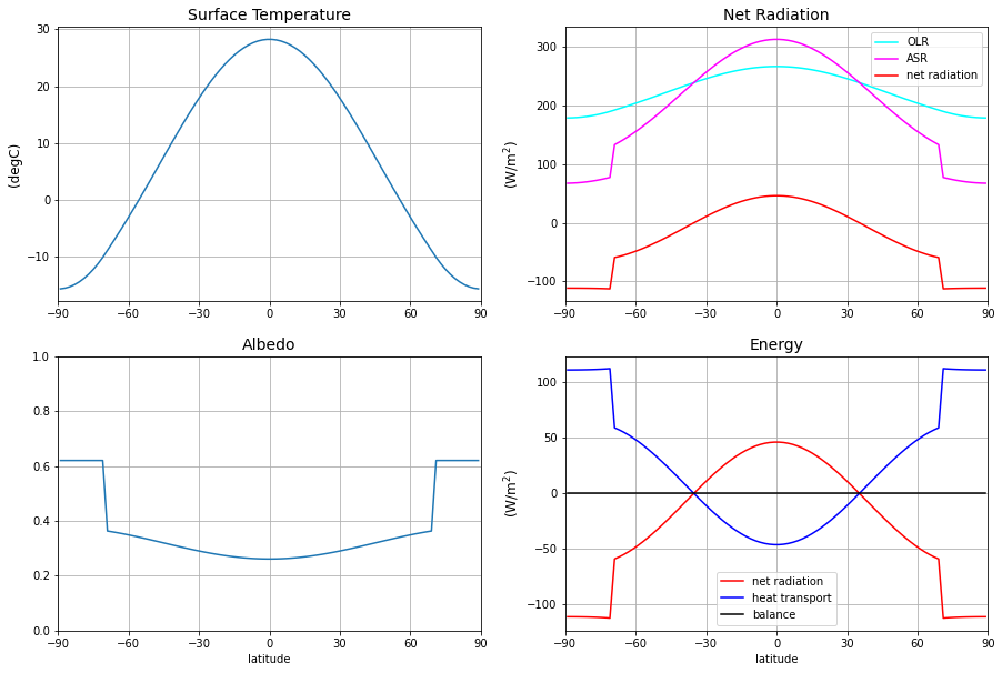
The energy balance is zero at every latitude. That means the model is in equilibrium. Perfect!
Global mean temperature
The model’s state dictionary has following entries:
[17]:
ebm_model.state.keys()
[17]:
dict_keys(['Ts'])
Like diagnostics, state variables can be accessed in two ways:
With dictionary methods,
ebm_model.state['Ts']As process attributes,
ebm_model.Ts
These are entirely equivalent:
[18]:
ebm_model.Ts is ebm_model.state['Ts']
[18]:
True
The global mean of the model’s surface temperature can be calculated through
[19]:
print('The global mean temperature is %.2f deg C.' %climlab.global_mean(ebm_model.Ts))
print('The modeled ice edge is at %.2f deg latitude.' %np.max(ebm_model.icelat))
The global mean temperature is 14.29 deg C.
The modeled ice edge is at 70.00 deg latitude.
[ ]: