Latitude-dependent grey radiation
Here is a quick example of using the climlab.GreyRadiationModel with a latitude dimension and seasonally varying insolation.
[1]:
%matplotlib inline
import numpy as np
import matplotlib.pyplot as plt
import climlab
from climlab import constants as const
[2]:
model = climlab.GreyRadiationModel(name='Grey Radiation', num_lev=30, num_lat=90)
print(model)
climlab Process of type <class 'climlab.model.column.GreyRadiationModel'>.
State variables and domain shapes:
  Ts: (90, 1)
  Tatm: (90, 30)
The subprocess tree:
Grey Radiation: <class 'climlab.model.column.GreyRadiationModel'>
   LW: <class 'climlab.radiation.greygas.GreyGas'>
   SW: <class 'climlab.radiation.greygas.GreyGasSW'>
   insolation: <class 'climlab.radiation.insolation.FixedInsolation'>
[3]:
model.to_xarray()
[3]:
<xarray.Dataset>
Dimensions:       (depth: 1, depth_bounds: 2, lat: 90, lat_bounds: 91, lev: 30, lev_bounds: 31)
Coordinates:
  * lat           (lat) float64 -89.0 -87.0 -85.0 -83.0 ... 83.0 85.0 87.0 89.0
  * depth         (depth) float64 0.5
  * lat_bounds    (lat_bounds) float64 -90.0 -88.0 -86.0 ... 86.0 88.0 90.0
  * depth_bounds  (depth_bounds) float64 0.0 1.0
  * lev           (lev) float64 16.67 50.0 83.33 116.7 ... 916.7 950.0 983.3
  * lev_bounds    (lev_bounds) float64 0.0 33.33 66.67 ... 933.3 966.7 1e+03
Data variables:
    Ts            (lat, depth) float64 288.0 288.0 288.0 ... 288.0 288.0 288.0
    Tatm          (lat, lev) float64 200.0 202.7 205.4 ... 272.6 275.3 278.0
xarray.Dataset
- depth: 1
- depth_bounds: 2
- lat: 90
- lat_bounds: 91
- lev: 30
- lev_bounds: 31
- lat(lat)float64-89.0 -87.0 -85.0 ... 87.0 89.0
- units :
- degrees
array([-89., -87., -85., -83., -81., -79., -77., -75., -73., -71., -69., -67., -65., -63., -61., -59., -57., -55., -53., -51., -49., -47., -45., -43., -41., -39., -37., -35., -33., -31., -29., -27., -25., -23., -21., -19., -17., -15., -13., -11., -9., -7., -5., -3., -1., 1., 3., 5., 7., 9., 11., 13., 15., 17., 19., 21., 23., 25., 27., 29., 31., 33., 35., 37., 39., 41., 43., 45., 47., 49., 51., 53., 55., 57., 59., 61., 63., 65., 67., 69., 71., 73., 75., 77., 79., 81., 83., 85., 87., 89.]) - depth(depth)float640.5
- units :
- meters
array([0.5])
- lat_bounds(lat_bounds)float64-90.0 -88.0 -86.0 ... 88.0 90.0
- units :
- degrees
array([-90., -88., -86., -84., -82., -80., -78., -76., -74., -72., -70., -68., -66., -64., -62., -60., -58., -56., -54., -52., -50., -48., -46., -44., -42., -40., -38., -36., -34., -32., -30., -28., -26., -24., -22., -20., -18., -16., -14., -12., -10., -8., -6., -4., -2., 0., 2., 4., 6., 8., 10., 12., 14., 16., 18., 20., 22., 24., 26., 28., 30., 32., 34., 36., 38., 40., 42., 44., 46., 48., 50., 52., 54., 56., 58., 60., 62., 64., 66., 68., 70., 72., 74., 76., 78., 80., 82., 84., 86., 88., 90.]) - depth_bounds(depth_bounds)float640.0 1.0
- units :
- meters
array([0., 1.])
- lev(lev)float6416.67 50.0 83.33 ... 950.0 983.3
- units :
- mb
array([ 16.666667, 50. , 83.333333, 116.666667, 150. , 183.333333, 216.666667, 250. , 283.333333, 316.666667, 350. , 383.333333, 416.666667, 450. , 483.333333, 516.666667, 550. , 583.333333, 616.666667, 650. , 683.333333, 716.666667, 750. , 783.333333, 816.666667, 850. , 883.333333, 916.666667, 950. , 983.333333]) - lev_bounds(lev_bounds)float640.0 33.33 66.67 ... 966.7 1e+03
- units :
- mb
array([   0.      ,   33.333333,   66.666667,  100.      ,  133.333333,
        166.666667,  200.      ,  233.333333,  266.666667,  300.      ,
        333.333333,  366.666667,  400.      ,  433.333333,  466.666667,
        500.      ,  533.333333,  566.666667,  600.      ,  633.333333,
        666.666667,  700.      ,  733.333333,  766.666667,  800.      ,
        833.333333,  866.666667,  900.      ,  933.333333,  966.666667,
       1000.      ])
- Ts(lat, depth)float64288.0 288.0 288.0 ... 288.0 288.0
array([[288.], [288.], [288.], [288.], [288.], [288.], [288.], [288.], [288.], [288.], [288.], [288.], [288.], [288.], [288.], [288.], [288.], [288.], [288.], [288.], ... [288.], [288.], [288.], [288.], [288.], [288.], [288.], [288.], [288.], [288.], [288.], [288.], [288.], [288.], [288.], [288.], [288.], [288.], [288.], [288.]]) - Tatm(lat, lev)float64200.0 202.7 205.4 ... 275.3 278.0
array([[200.        , 202.68965517, 205.37931034, ..., 272.62068966,
        275.31034483, 278.        ],
       [200.        , 202.68965517, 205.37931034, ..., 272.62068966,
        275.31034483, 278.        ],
       [200.        , 202.68965517, 205.37931034, ..., 272.62068966,
        275.31034483, 278.        ],
       ...,
       [200.        , 202.68965517, 205.37931034, ..., 272.62068966,
        275.31034483, 278.        ],
       [200.        , 202.68965517, 205.37931034, ..., 272.62068966,
        275.31034483, 278.        ],
       [200.        , 202.68965517, 205.37931034, ..., 272.62068966,
        275.31034483, 278.        ]])
[4]:
insolation = climlab.radiation.DailyInsolation(domains=model.Ts.domain)
[5]:
model.add_subprocess('insolation', insolation)
model.subprocess.SW.flux_from_space = insolation.insolation
[6]:
print(model)
climlab Process of type <class 'climlab.model.column.GreyRadiationModel'>.
State variables and domain shapes:
  Ts: (90, 1)
  Tatm: (90, 30)
The subprocess tree:
Grey Radiation: <class 'climlab.model.column.GreyRadiationModel'>
   LW: <class 'climlab.radiation.greygas.GreyGas'>
   SW: <class 'climlab.radiation.greygas.GreyGasSW'>
   insolation: <class 'climlab.radiation.insolation.DailyInsolation'>
[7]:
model.compute_diagnostics()
[8]:
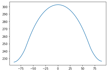
plt.plot(model.lat, model.SW_down_TOA)
[8]:
[<matplotlib.lines.Line2D at 0x16c3f65e0>]
[9]:
model.Tatm.shape
[9]:
(90, 30)
[10]:
model.integrate_years(1)
Integrating for 365 steps, 365.2422 days, or 1 years.
Total elapsed time is 0.9993368783782377 years.
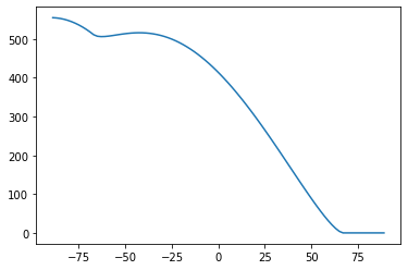
[11]:
plt.plot(model.lat, model.Ts)
[11]:
[<matplotlib.lines.Line2D at 0x16c4f2070>]
[12]:
model.integrate_years(1)
Integrating for 365 steps, 365.2422 days, or 1 years.
Total elapsed time is 1.9986737567564754 years.
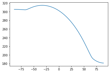
[13]:
plt.plot(model.lat, model.timeave['Ts'])
[13]:
[<matplotlib.lines.Line2D at 0x16c562910>]
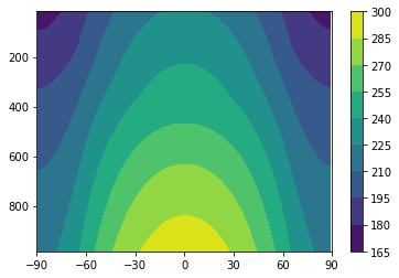
[14]:
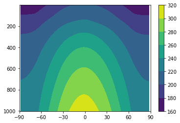
def plot_temp_section(model, timeave=True):
    fig = plt.figure()
    ax = fig.add_subplot(111)
    if timeave:
        field = model.timeave['Tatm'].transpose()
    else:
        field = model.Tatm.transpose()
    cax = ax.contourf(model.lat, model.lev, field)
    ax.invert_yaxis()
    ax.set_xlim(-90,90)
    ax.set_xticks([-90, -60, -30, 0, 30, 60, 90])
    fig.colorbar(cax)
[15]:
plot_temp_section(model)

[16]:
model2 = climlab.RadiativeConvectiveModel(name='RCM', num_lev=30, num_lat=90)
insolation = climlab.radiation.DailyInsolation(domains=model2.Ts.domain)
model2.add_subprocess('insolation', insolation)
model2.subprocess.SW.flux_from_space = insolation.insolation
[17]:
model2.integrate_years(1)
Integrating for 365 steps, 365.2422 days, or 1 years.
Total elapsed time is 0.9993368783782377 years.
[18]:
model2.integrate_years(1)
Integrating for 365 steps, 365.2422 days, or 1 years.
Total elapsed time is 1.9986737567564754 years.
[19]:
plot_temp_section(model2)

Testing out multi-dimensional Band Models
[20]:
#  Put in some ozone
import xarray as xr

ozonepath = "http://thredds.atmos.albany.edu:8080/thredds/dodsC/CLIMLAB/ozone/apeozone_cam3_5_54.nc"
ozone = xr.open_dataset(ozonepath)
ozone
[20]:
<xarray.Dataset>
Dimensions:    (lat: 64, lev: 59, lon: 128, time: 12)
Coordinates:
  * lev        (lev) float64 0.2842 0.3253 0.3719 ... 849.5 959.0 1.004e+03
  * lon        (lon) float64 0.0 2.812 5.625 8.438 ... 348.8 351.6 354.4 357.2
  * lat        (lat) float64 -87.86 -85.1 -82.31 -79.53 ... 82.31 85.1 87.86
  * time       (time) float64 4.382e+04 4.384e+04 ... 4.412e+04 4.415e+04
Data variables:
    P0         float64 1.004e+05
    date       (time) int32 19900116 19900214 19900316 ... 19901115 19901216
    datesec    (time) int32 0 0 0 0 0 0 0 0 0 0 0 0
    OZONE_old  (time, lat, lev, lon) float64 ...
    OZONE      (time, lev, lat, lon) float64 ...
Attributes:
    Conventions:                     NCAR-CSM
    Source:                          AMIP II (symmetric for APE project)
    Written_By:                      olson
    Date_Written:                    August 22 2003
    Host:                            zen
    Command:                         ncgen
    history:                         Wed Jul 30 08:35:58 2008: ncrename -v OZ...
    DODS_EXTRA.Unlimited_Dimension:  time
xarray.Dataset
- lat: 64
- lev: 59
- lon: 128
- time: 12
- lev(lev)float640.2842 0.3253 ... 959.0 1.004e+03
- long_name :
- hybrid level at layer midpoints (1000*(A+B))
- units :
- hybrid_sigma_pressure
- positive :
- down
array([2.84191e-01, 3.25350e-01, 3.71936e-01, 4.24615e-01, 4.84153e-01, 5.51432e-01, 6.27490e-01, 7.13542e-01, 8.11039e-01, 9.21699e-01, 1.04757e+00, 1.19108e+00, 1.35511e+00, 1.54305e+00, 1.75891e+00, 2.00739e+00, 2.29403e+00, 2.62529e+00, 3.00884e+00, 3.45369e+00, 3.97050e+00, 4.57190e+00, 5.27278e+00, 6.09073e+00, 7.04636e+00, 8.16371e+00, 9.47075e+00, 1.10000e+01, 1.27894e+01, 1.48832e+01, 1.73342e+01, 2.02039e+01, 2.35659e+01, 2.75066e+01, 3.21283e+01, 3.75509e+01, 4.39150e+01, 5.13840e+01, 6.01483e+01, 7.04289e+01, 8.24830e+01, 9.66096e+01, 1.13155e+02, 1.32514e+02, 1.55122e+02, 1.81445e+02, 2.11947e+02, 2.47079e+02, 2.87273e+02, 3.32956e+02, 3.84573e+02, 4.42610e+02, 5.07601e+02, 5.80132e+02, 6.60837e+02, 7.50393e+02, 8.49521e+02, 9.58981e+02, 1.00369e+03]) - lon(lon)float640.0 2.812 5.625 ... 354.4 357.2
- long_name :
- longitude
- units :
- degrees_east
array([ 0. , 2.8125, 5.625 , 8.4375, 11.25 , 14.0625, 16.875 , 19.6875, 22.5 , 25.3125, 28.125 , 30.9375, 33.75 , 36.5625, 39.375 , 42.1875, 45. , 47.8125, 50.625 , 53.4375, 56.25 , 59.0625, 61.875 , 64.6875, 67.5 , 70.3125, 73.125 , 75.9375, 78.75 , 81.5625, 84.375 , 87.1875, 90. , 92.8125, 95.625 , 98.4375, 101.25 , 104.0625, 106.875 , 109.6875, 112.5 , 115.3125, 118.125 , 120.9375, 123.75 , 126.5625, 129.375 , 132.1875, 135. , 137.8125, 140.625 , 143.4375, 146.25 , 149.0625, 151.875 , 154.6875, 157.5 , 160.3125, 163.125 , 165.9375, 168.75 , 171.5625, 174.375 , 177.1875, 180. , 182.8125, 185.625 , 188.4375, 191.25 , 194.0625, 196.875 , 199.6875, 202.5 , 205.3125, 208.125 , 210.9375, 213.75 , 216.5625, 219.375 , 222.1875, 225. , 227.8125, 230.625 , 233.4375, 236.25 , 239.0625, 241.875 , 244.6875, 247.5 , 250.3125, 253.125 , 255.9375, 258.75 , 261.5625, 264.375 , 267.1875, 270. , 272.8125, 275.625 , 278.4375, 281.25 , 284.0625, 286.875 , 289.6875, 292.5 , 295.3125, 298.125 , 300.9375, 303.75 , 306.5625, 309.375 , 312.1875, 315. , 317.8125, 320.625 , 323.4375, 326.25 , 329.0625, 331.875 , 334.6875, 337.5 , 340.3125, 343.125 , 345.9375, 348.75 , 351.5625, 354.375 , 357.1875]) - lat(lat)float64-87.86 -85.1 -82.31 ... 85.1 87.86
- long_name :
- latitude
- units :
- degrees_north
array([-87.8638, -85.0965, -82.3129, -79.5256, -76.7369, -73.9475, -71.1577, -68.3678, -65.5776, -62.7873, -59.997 , -57.2066, -54.4162, -51.6257, -48.8352, -46.0447, -43.2542, -40.4636, -37.6731, -34.8825, -32.0919, -29.3014, -26.5108, -23.7202, -20.9296, -18.139 , -15.3484, -12.5578, -9.7671, -6.9765, -4.1859, -1.3953, 1.3953, 4.1859, 6.9765, 9.7671, 12.5578, 15.3484, 18.139 , 20.9296, 23.7202, 26.5108, 29.3014, 32.0919, 34.8825, 37.6731, 40.4636, 43.2542, 46.0447, 48.8352, 51.6257, 54.4162, 57.2066, 59.997 , 62.7873, 65.5776, 68.3678, 71.1577, 73.9475, 76.7369, 79.5256, 82.3129, 85.0965, 87.8638]) - time(time)float644.382e+04 4.384e+04 ... 4.415e+04
- long_name :
- time
- units :
- day number (Jan 1 = 1)
- calendar :
- 365_days
array([43816., 43844., 43875., 43905., 43936., 43966., 43997., 44028., 44058.,
       44089., 44119., 44150.])
- P0()float64...
- long_name :
- reference pressure
- units :
- Pa
array(100369.)
- date(time)int32...
- long_name :
- current date as 8 digit integer (YYYYMMDD)
array([19900116, 19900214, 19900316, 19900415, 19900516, 19900615, 19900716, 19900816, 19900915, 19901016, 19901115, 19901216], dtype=int32) - datesec(time)int32...
- long_name :
- seconds of current date
- units :
- s
array([0, 0, 0, 0, 0, 0, 0, 0, 0, 0, 0, 0], dtype=int32)
- OZONE_old(time, lat, lev, lon)float64...
- long_name :
- OZONE
- units :
- FRACTION
[5799936 values with dtype=float64]
- OZONE(time, lev, lat, lon)float64...
- long_name :
- OZONE
- units :
- FRACTION
[5799936 values with dtype=float64]
- Conventions :
- NCAR-CSM
- Source :
- AMIP II (symmetric for APE project)
- Written_By :
- olson
- Date_Written :
- August 22 2003
- Host :
- zen
- Command :
- ncgen
- history :
- Wed Jul 30 08:35:58 2008: ncrename -v OZONE,OZONE_old apeozone_cam3_5_54.nc
- DODS_EXTRA.Unlimited_Dimension :
- time
[21]:
#  Dimensions of the ozone file
lat = ozone.lat
lon = ozone.lon
lev = ozone.lev

# Taking annual, zonal average of the ozone data
O3_zon = ozone.OZONE.mean(dim=("time","lon"))
[22]:
#  make a model on the same grid as the ozone
model3 = climlab.BandRCModel(model='Band RCM', lev=lev, lat=lat)
insolation = climlab.radiation.DailyInsolation(domains=model3.Ts.domain)
model3.add_subprocess('insolation', insolation)
model3.subprocess.SW.flux_from_space = insolation.insolation
print(model3)
climlab Process of type <class 'climlab.model.column.BandRCModel'>.
State variables and domain shapes:
  Ts: (64, 1)
  Tatm: (64, 59)
The subprocess tree:
Untitled: <class 'climlab.model.column.BandRCModel'>
   LW: <class 'climlab.radiation.nband.FourBandLW'>
   SW: <class 'climlab.radiation.nband.ThreeBandSW'>
   insolation: <class 'climlab.radiation.insolation.DailyInsolation'>
   convective adjustment: <class 'climlab.convection.convadj.ConvectiveAdjustment'>
   H2O: <class 'climlab.radiation.water_vapor.ManabeWaterVapor'>
[23]:
# Put in the ozone
model3.absorber_vmr['O3'] = O3_zon.transpose()
[24]:
print(model3.absorber_vmr['O3'].shape)
print(model3.Tatm.shape)
(64, 59)
(64, 59)
[25]:
model3.step_forward()
[26]:
model3.integrate_years(1.)
Integrating for 365 steps, 365.2422 days, or 1.0 years.
Total elapsed time is 1.0020747876340685 years.
[27]:
model3.integrate_years(1.)
Integrating for 365 steps, 365.2422 days, or 1.0 years.
Total elapsed time is 2.0014116660123062 years.
[28]:
plot_temp_section(model3)
This is now working. Will need to do some model tuning.
And start to add dynamics!
Adding meridional diffusion!
[29]:
print(model2)
climlab Process of type <class 'climlab.model.column.RadiativeConvectiveModel'>.
State variables and domain shapes:
  Ts: (90, 1)
  Tatm: (90, 30)
The subprocess tree:
RCM: <class 'climlab.model.column.RadiativeConvectiveModel'>
   LW: <class 'climlab.radiation.greygas.GreyGas'>
   SW: <class 'climlab.radiation.greygas.GreyGasSW'>
   insolation: <class 'climlab.radiation.insolation.DailyInsolation'>
   convective adjustment: <class 'climlab.convection.convadj.ConvectiveAdjustment'>
[30]:
diffmodel = climlab.process_like(model2)
diffmodel.name = "RCM with heat transport"
[31]:
# thermal diffusivity in W/m**2/degC
D = 0.05
# meridional diffusivity in m**2/s
K = D / diffmodel.Tatm.domain.heat_capacity[0] * const.a**2
print(K)
5946637.413346613
[32]:
d = climlab.dynamics.MeridionalDiffusion(K=K, state={'Tatm': diffmodel.Tatm}, **diffmodel.param)
[33]:
diffmodel.add_subprocess('diffusion', d)
[34]:
print(diffmodel)
climlab Process of type <class 'climlab.model.column.RadiativeConvectiveModel'>.
State variables and domain shapes:
  Ts: (90, 1)
  Tatm: (90, 30)
The subprocess tree:
RCM with heat transport: <class 'climlab.model.column.RadiativeConvectiveModel'>
   LW: <class 'climlab.radiation.greygas.GreyGas'>
   SW: <class 'climlab.radiation.greygas.GreyGasSW'>
   insolation: <class 'climlab.radiation.insolation.DailyInsolation'>
   convective adjustment: <class 'climlab.convection.convadj.ConvectiveAdjustment'>
   diffusion: <class 'climlab.dynamics.meridional_advection_diffusion.MeridionalDiffusion'>
[35]:
diffmodel.step_forward()
[36]:
diffmodel.integrate_years(1)
Integrating for 365 steps, 365.2422 days, or 1 years.
Total elapsed time is 3.000748544390544 years.
[37]:
diffmodel.integrate_years(1)
Integrating for 365 steps, 365.2422 days, or 1 years.
Total elapsed time is 4.000085422768781 years.
[38]:
plot_temp_section(model2)
plot_temp_section(diffmodel)

This works as long as K is a constant.
The diffusion operation is broadcast over all vertical levels without any special code.
[39]:
def inferred_heat_transport( energy_in, lat_deg ):
    '''Returns the inferred heat transport (in PW) by integrating the net energy imbalance from pole to pole.'''
    from scipy import integrate
    from climlab import constants as const
    lat_rad = np.deg2rad( lat_deg )
    return ( 1E-15 * 2 * np.math.pi * const.a**2 * integrate.cumtrapz( np.cos(lat_rad)*energy_in,
            x=lat_rad, initial=0. ) )
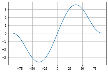
[40]:
#  Plot the northward heat transport in this model
Rtoa = np.squeeze(diffmodel.timeave['ASR'] - diffmodel.timeave['OLR'])
plt.plot(diffmodel.lat, inferred_heat_transport(Rtoa, diffmodel.lat))
plt.grid()
Band model with diffusion
[41]:
diffband = climlab.process_like(model3)
diffband.name = "Band RCM with heat transport"
[42]:
d = climlab.dynamics.MeridionalDiffusion(K=K, state={'Tatm': diffband.Tatm}, **diffband.param)
diffband.add_subprocess('diffusion', d)
print(diffband)
climlab Process of type <class 'climlab.model.column.BandRCModel'>.
State variables and domain shapes:
  Ts: (64, 1)
  Tatm: (64, 59)
The subprocess tree:
Band RCM with heat transport: <class 'climlab.model.column.BandRCModel'>
   LW: <class 'climlab.radiation.nband.FourBandLW'>
   SW: <class 'climlab.radiation.nband.ThreeBandSW'>
   insolation: <class 'climlab.radiation.insolation.DailyInsolation'>
   convective adjustment: <class 'climlab.convection.convadj.ConvectiveAdjustment'>
   H2O: <class 'climlab.radiation.water_vapor.ManabeWaterVapor'>
   diffusion: <class 'climlab.dynamics.meridional_advection_diffusion.MeridionalDiffusion'>
[43]:
diffband.integrate_years(1)
Integrating for 365 steps, 365.2422 days, or 1 years.
Total elapsed time is 3.000748544390544 years.
[44]:
diffband.integrate_years(1)
Integrating for 365 steps, 365.2422 days, or 1 years.
Total elapsed time is 4.000085422768781 years.
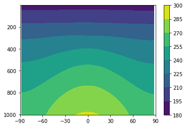
[45]:
plot_temp_section(model3)
plot_temp_section(diffband)

[46]:
plt.plot(diffband.lat, diffband.timeave['ASR'] - diffband.timeave['OLR'])
[46]:
[<matplotlib.lines.Line2D at 0x16d30c550>]
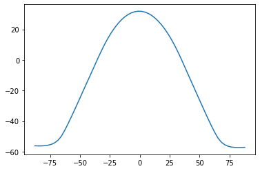
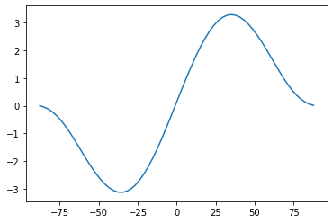
[47]:
#  Plot the northward heat transport in this model
Rtoa = np.squeeze(diffband.timeave['ASR'] - diffband.timeave['OLR'])
plt.plot(diffband.lat, inferred_heat_transport(Rtoa, diffband.lat))
[47]:
[<matplotlib.lines.Line2D at 0x16d36ad00>]
[ ]: