ebm

Inheritance diagram of climlab.model.ebm

Convenience classes for pre-made Energy Balance Models in CLIMLAB.

These models all solve some form of the equation

\[C \frac{\partial}{\partial t} T_s(\phi,t) = (1-\alpha)S(\phi,t) - \left[A + B T_s \right] + \frac{1}{\cos\phi} \frac{\partial}{\partial \phi} \left[ \cos\phi ~ D ~ \frac{\partial T_s}{\partial \phi} \right]\]

where

\(\phi\) is latitude
\(T_s\) is a zonally averaged surface temperature
\(C\) is a depth-integrated heat capacity
\(\alpha\) is an albedo (which may depend on latitude and/or temperature)
\(S(\phi, t)\) is the insolation
\(\left[A + B T_s \right]\) is a parameterization of the Outgoing Longwave Radiation to space
the last term on the right hand side is a diffusive heat transport convergence with thermal diffusivity \(D\) in the same units as \(B\)

Three classes are provided, which differ in the type of insolation \(S\):

climlab.EBM uses a steady idealized annual insolation (second Legendre polynomial form)
climlab.EBM_annual uses realistic steady annual-mean insolation
climlab.EBM_seasonal uses realistic seasonally varying insolation

The __init__ method of class EBM shows how these models are assembled from subprocesses representing each term in the above equation.

Building the Moist EBM

There is currently no ready-made convenience class for the moist EBM, but it can be readily built by swapping out the dry heat diffusion process climlab.dynamics.MeridionalHeatDiffusion with the moist equivalent climlab.dynamics.MeridionalMoistDiffusion.

This sort of mixing and matching of model components is at the heart of CLIMLAB design and functionality.

Example:

import climlab
#  create and display a 1D Energy Balance Model
dry = climlab.EBM()
print(dry)
#  clone this model and swap out the diffusion subprocess
moist = climlab.process_like(dry)
diff = climlab.dynamics.MeridionalMoistDiffusion(state=moist.state, timestep=moist.timestep)
moist.add_subprocess('diffusion', diff)
print(moist)

We can run both models out to equilibrium and compare the results as follows:

Example:

#  Run both models out to quasi-equilibrium
#   print out the global mean planetary energy budget -- should be very small
for m in [dry, moist]:
    m.integrate_years(10)
    print(climlab.global_mean(m.net_radiation))
#  plot and compare the temperatures
import matplotlib.pyplot as plt
plt.figure()
plt.plot(dry.lat, dry.Ts, label='Dry')
plt.plot(moist.lat, moist.Ts, label='Moist')
plt.legend()
plt.show()
#  plot and compare the heat transport
plt.figure()
plt.plot(dry.lat_bounds, dry.heat_transport, label='Dry')
plt.plot(moist.lat_bounds, moist.heat_transport, label='Moist')
plt.legend()
plt.show()

class climlab.model.ebm.EBM(num_lat=90, num_lon=None, S0=1365.2, s2=-0.48, A=210.0, B=2.0, D=0.555, water_depth=10.0, Tf=-10.0, a0=0.3, a2=0.078, ai=0.62, timestep=350632.51200000005, initial_time=np.datetime64('1970-01-01T00:00'), T0=12.0, T2=-40.0, **kwargs)[source]

Bases: TimeDependentProcess

A parent class for all Energy-Balance-Model classes.

This class sets up a typical EnergyBalance Model with following subprocesses:

Outgoing Longwave Radiation (OLR) parametrization through AplusBT
Absorbed Shortwave Radiation (ASR) through SimpleAbsorbedShortwave
solar insolation paramtrization through P2Insolation
albedo parametrization in dependence of temperature through StepFunctionAlbedo
energy diffusion through MeridionalHeatDiffusion

Initialization parameters n

An instance of EBM is initialized with the following arguments (for detailed information see Object attributes below):

Parameters:

num_lat (int) –
number of equally spaced points for the latitue grid. Used for domain intialization of zonal_mean_surface
- default value: 90
num_lon (int) –
number of equally spaced points in longitude
- default value: None
S0 (float) – solar constant - unit: \(\frac{\textrm{W}}{\textrm{m}^2}\) - default value: 1365.2
A (float) – parameter for linear OLR parametrization AplusBT - unit: \(\frac{\textrm{W}}{\textrm{m}^2}\) - default value: 210.0
B (float) – parameter for linear OLR parametrization AplusBT - unit: \(\frac{\textrm{W}}{\textrm{m}^2 ~ ^{\circ} \textrm{C}}\) - default value: 2.0
D (float) –
diffusion parameter for Meridional Energy Diffusion MeridionalDiffusion
- unit: \(\frac{\textrm{W}}{\textrm{m}^2 ~ ^{\circ} \textrm{C}}\)
- default value: 0.555
water_depth (float) –
depth of zonal_mean_surface domain, which the heat capacity is dependent on
- unit: meters
- default value: 10.0
Tf (float) – freezing temperature - unit: \(^{\circ} \textrm{C}\) - default value: -10.0
a0 (float) –
base value for planetary albedo parametrization StepFunctionAlbedo
- unit: dimensionless
- default value: 0.3
a2 (float) –
parabolic value for planetary albedo parametrization StepFunctionAlbedo
- unit: dimensionless
- default value: 0.078
ai (float) –
value for ice albedo paramerization in StepFunctionAlbedo
- unit: dimensionless
- default value: 0.62
timestep (float) –
specifies the EBM’s timestep - unit: seconds - default value: (365.2422 * 24 * 60 * 60 ) / 90

-> (90 timesteps per year)
T0 (float) – base value for initial temperature - unit \(^{\circ} \textrm{C}\) - default value: 12
T2 (float) – factor for 2nd Legendre polynomial P2 to calculate initial temperature - unit: dimensionless - default value: 40

Object attributes n

Additional to the parent class EnergyBudget following object attributes are generated and updated during initialization:

Variables:

param (dict) – The parameter dictionary is updated with a couple of the initatilzation input arguments, namely 'S0', 'A', 'B', 'D', 'Tf', 'water_depth', 'a0', 'a2' and 'ai'.
domains (dict) – If the object’s domains and the state dictionaries are empty during initialization a domain sfc is created through zonal_mean_surface(). In the meantime the object’s domains and state dictionaries are updated.
subprocess (dict) – Several subprocesses are created (see above) through calling add_subprocess() and therefore the subprocess dictionary is updated.
topdown (bool) – is set to False to call subprocess compute methods first. See also TimeDependentProcess.
diagnostics (dict) – is initialized with keys: 'OLR', 'ASR', 'net_radiation', 'albedo', 'icelat' and 'ice_area' through add_diagnostic().

Example:

Creation and integration of the preconfigured Energy Balance Model:

>>> import climlab
>>> model = climlab.EBM()

>>> model.integrate_years(2.)
Integrating for 180 steps, 730.4844 days, or 2.0 years.
Total elapsed time is 2.0 years.

For more information how to use the EBM class, see the Tutorials chapter.

Attributes:

S0
current_time
depth: Depth at grid centers (m)
depth_bounds: Depth at grid interfaces (m)
diagnostics: Dictionary access to all diagnostic variables
elapsed_time
input: Dictionary access to all input variables
lat: Latitude of grid centers (degrees North)
lat_bounds: Latitude of grid interfaces (degrees North)
lev: Pressure levels at grid centers (hPa or mb)
lev_bounds: Pressure levels at grid interfaces (hPa or mb)
lon: Longitude of grid centers (degrees)
lon_bounds: Longitude of grid interfaces (degrees)
timestep: The amount of time over which step_forward() is integrating in unit seconds.
timestep_in_seconds: Return a float value representing the timestep in units of seconds

Methods

`add_diagnostic`(name[, value])	Create a new diagnostic variable called `name` for this process and initialize it with the given `value`.
`add_input`(name[, value])	Create a new input variable called `name` for this process and initialize it with the given `value`.
`add_subprocess`(name, proc[, verbose])	Adds a single subprocess to this process.
`add_subprocesses`(procdict)	Adds a dictionary of subproceses to this process.
`compute`()	Computes the tendencies for all state variables given current state and specified input.
`compute_diagnostics`([num_iter])	Compute all tendencies and diagnostics, but don't update model state.
`declare_diagnostics`(diaglist)	Add the variable names in `inputlist` to the list of diagnostics.
`declare_input`(inputlist)	Add the variable names in `inputlist` to the list of necessary inputs.
`diffusive_heat_transport`()	Compute instantaneous diffusive heat transport in unit \(\textrm{PW}\) on the staggered grid (bounds) through calculating:
`global_mean_temperature`()	Convenience method to compute global mean surface temperature.
`inferred_heat_transport`()	Calculates the inferred heat transport by integrating the TOA energy imbalance from pole to pole.
`integrate_converge`([crit, verbose])	Integrates the model until model states are converging.
`integrate_days`([days, verbose])	Integrates the model forward for a specified number of days.
`integrate_years`([years, verbose])	Integrates the model by a given number of years.
`remove_diagnostic`(name)	Removes a diagnostic from the `process.diagnostic` dictionary and also delete the associated process attribute.
`remove_subprocess`(name[, verbose])	Removes a single subprocess from this process.
`set_state`(name, value)	Sets the variable `name` to a new state `value`.
`step_forward`()	Updates state variables with computed tendencies.
`to_xarray`([diagnostics, timeave])	Convert process variables to `xarray.Dataset` format.

property S0

diffusive_heat_transport()[source]

Compute instantaneous diffusive heat transport in unit \(\textrm{PW}\) on the staggered grid (bounds) through calculating:

\[H(\varphi) = - 2 \pi R^2 cos(\varphi) D \frac{dT}{d\varphi} \approx - 2 \pi R^2 cos(\varphi) D \frac{\Delta T}{\Delta \varphi}\]

Return type:: array of size np.size(self.lat_bounds)

THIS IS DEPRECATED AND WILL BE REMOVED IN THE FUTURE. Use the diagnostic heat_transport instead, which implements the same calculation.

global_mean_temperature()[source]

Convenience method to compute global mean surface temperature.

Calls global_mean() method which for the object attriute Ts which calculates the latitude weighted global mean of a field.

Example:

Calculating the global mean temperature of initial EBM temperature:

>>> import climlab
>>> model = climlab.EBM(T0=14., T2=-25)

>>> model.global_mean_temperature()
Field(13.99873037400856)

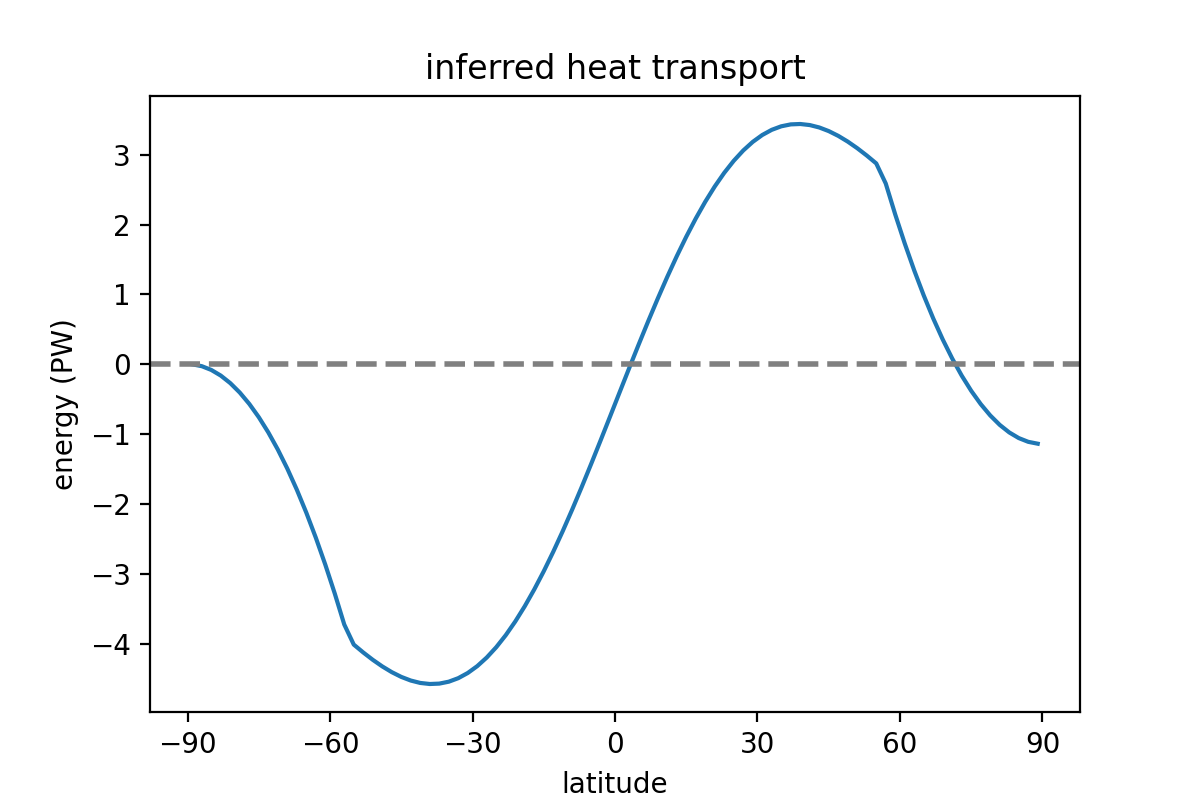
inferred_heat_transport()[source]

Calculates the inferred heat transport by integrating the TOA energy imbalance from pole to pole.

The method is calculating

\[H(\varphi) = 2 \pi R^2 \int_{-\pi/2}^{\varphi} cos\phi \ R_{TOA} d\phi\]

where \(R_{TOA}\) is the net radiation at top of atmosphere.

Returns:

total heat transport on the latitude grid in unit \(\textrm{PW}\)

Return type:

array of size np.size(self.lat_lat)

Example:

import climlab
import matplotlib.pyplot as plt

# creating & integrating model
model = climlab.EBM()
model.step_forward()

# plot
fig = plt.figure( figsize=(6,4))
ax = fig.add_subplot(111)

ax.plot(model.lat, model.inferred_heat_transport())

ax.set_title('inferred heat transport')
ax.set_xlabel('latitude')
ax.set_xticks([-90,-60,-30,0,30,60,90])
ax.set_ylabel('energy (PW)')
plt.axhline(linewidth=2, color='grey', linestyle='dashed')
plt.show()

(Source code, png, hires.png, pdf)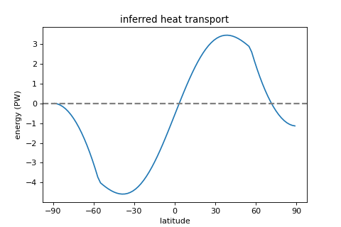

../_images/example_EBM_inferred_heat_transport.png

class climlab.model.ebm.EBM_annual(**kwargs)[source]

Bases: EBM_seasonal

A class that implements Energy Balance Models with annual mean insolation.

The annual solar distribution is calculated through averaging the DailyInsolation over time which has been used in used in the parent class EBM_seasonal. That is done by the subprocess AnnualMeanInsolation which is more realistic than the P2Insolation module used in the classical EBM class.

According to the parent class EBM_seasonal the model will not have an ice-albedo feedback, if albedo ice parameter 'ai' is not given. For details see there.

Object attributes n

Following object attributes are updated during initialization: n

Variables:

subprocess (dict) – suprocess 'insolation' is overwritten by AnnualMeanInsolation

Example:

The EBM_annual class uses a different insolation subprocess than the EBM class:

>>> import climlab
>>> model_annual = climlab.EBM_annual()

>>> print model_annual

 climlab Process of type <class 'climlab.model.ebm.EBM_annual'>.
 State variables and domain shapes:
   Ts: (90, 1)
 The subprocess tree:
 top: <class 'climlab.EBM_annual'>
    diffusion: <class 'climlab.dynamics.MeridionalHeatDiffusion'>
    LW: <class 'climlab.radiation.AplusBT'>
    albedo: <class 'climlab.surface.P2Albedo'>
    insolation: <class 'climlab.radiation.AnnualMeanInsolation'>

Attributes:

S0
current_time
depth: Depth at grid centers (m)
depth_bounds: Depth at grid interfaces (m)
diagnostics: Dictionary access to all diagnostic variables
elapsed_time
input: Dictionary access to all input variables
lat: Latitude of grid centers (degrees North)
lat_bounds: Latitude of grid interfaces (degrees North)
lev: Pressure levels at grid centers (hPa or mb)
lev_bounds: Pressure levels at grid interfaces (hPa or mb)
lon: Longitude of grid centers (degrees)
lon_bounds: Longitude of grid interfaces (degrees)
timestep: The amount of time over which step_forward() is integrating in unit seconds.
timestep_in_seconds: Return a float value representing the timestep in units of seconds

Methods

`add_diagnostic`(name[, value])	Create a new diagnostic variable called `name` for this process and initialize it with the given `value`.
`add_input`(name[, value])	Create a new input variable called `name` for this process and initialize it with the given `value`.
`add_subprocess`(name, proc[, verbose])	Adds a single subprocess to this process.
`add_subprocesses`(procdict)	Adds a dictionary of subproceses to this process.
`compute`()	Computes the tendencies for all state variables given current state and specified input.
`compute_diagnostics`([num_iter])	Compute all tendencies and diagnostics, but don't update model state.
`declare_diagnostics`(diaglist)	Add the variable names in `inputlist` to the list of diagnostics.
`declare_input`(inputlist)	Add the variable names in `inputlist` to the list of necessary inputs.
`diffusive_heat_transport`()	Compute instantaneous diffusive heat transport in unit \(\textrm{PW}\) on the staggered grid (bounds) through calculating:
`global_mean_temperature`()	Convenience method to compute global mean surface temperature.
`inferred_heat_transport`()	Calculates the inferred heat transport by integrating the TOA energy imbalance from pole to pole.
`integrate_converge`([crit, verbose])	Integrates the model until model states are converging.
`integrate_days`([days, verbose])	Integrates the model forward for a specified number of days.
`integrate_years`([years, verbose])	Integrates the model by a given number of years.
`remove_diagnostic`(name)	Removes a diagnostic from the `process.diagnostic` dictionary and also delete the associated process attribute.
`remove_subprocess`(name[, verbose])	Removes a single subprocess from this process.
`set_state`(name, value)	Sets the variable `name` to a new state `value`.
`step_forward`()	Updates state variables with computed tendencies.
`to_xarray`([diagnostics, timeave])	Convert process variables to `xarray.Dataset` format.

class climlab.model.ebm.EBM_seasonal(a0=0.33, a2=0.25, ai=None, **kwargs)[source]

Bases: EBM

A class that implements Energy Balance Models with realistic daily insolation.

This class is inherited from the general EBM class and uses the insolation subprocess DailyInsolation instead of P2Insolation to compute a realisitc distribution of solar radiation on a daily basis.

If argument for ice albedo 'ai' is not given, the model will not have an albedo feedback.

An instance of EBM_seasonal is initialized with the following arguments:

Parameters:

a0 (float) – base value for planetary albedo parametrization StepFunctionAlbedo [default: 0.33]
a2 (float) – parabolic value for planetary albedo parametrization StepFunctionAlbedo [default: 0.25]
ai (float) – value for ice albedo paramerization in StepFunctionAlbedo (optional)

Object attributes n

Following object attributes are updated during initialization: n

Variables:

param (dict) – The parameter dictionary is updated with 'a0' and 'a2'.
subprocess (dict) – suprocess 'insolation' is overwritten by DailyInsolation.

if 'ai' is not given:

Variables:

param (dict) – 'ai' and 'Tf' are removed from the parameter dictionary (initialized by parent class EBM)
subprocess (dict) – suprocess 'albedo' is overwritten by P2Albedo.

if 'ai' is given:

Variables:

param (dict) – The parameter dictionary is updated with 'ai'.
subprocess (dict) – suprocess 'albedo' is overwritten by StepFunctionAlbedo (which basically has been there before but now is updated with the new albedo parameter values).

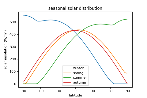
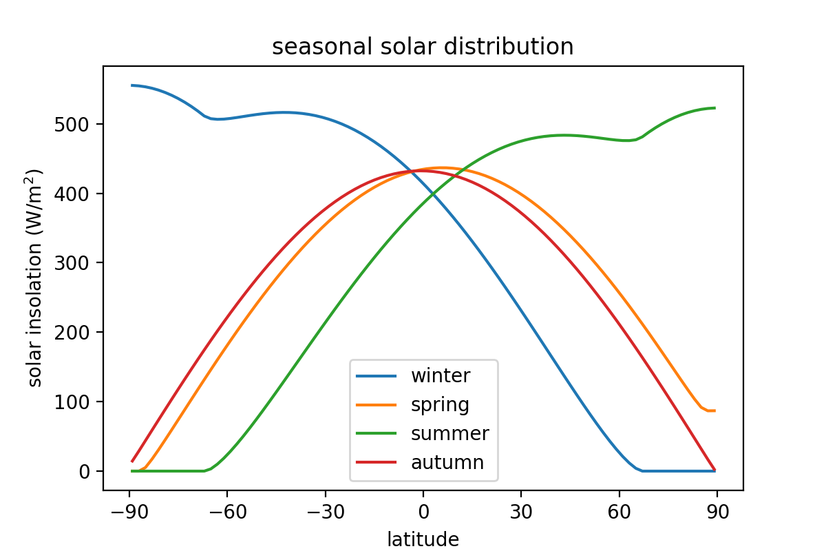
Example:

The annual distribution of solar insolation:

import climlab
from climlab.utils import constants as const
import numpy as np
import matplotlib.pyplot as plt

# creating model
model = climlab.EBM_seasonal()
model.step_forward()

solar = model.subprocess['insolation'].insolation

# plot
fig = plt.figure( figsize=(6,4))
ax = fig.add_subplot(111)

season_days = const.days_per_year/4

for season in ['winter','spring','summer','autumn']:
    ax.plot(model.lat, solar, label=season)
    model.integrate_days(season_days)

ax.set_title('seasonal solar distribution')
ax.set_xlabel('latitude')
ax.set_xticks([-90,-60,-30,0,30,60,90])
ax.set_ylabel('solar insolation (W/m$^2$)')
ax.legend(loc='best')
plt.show()

(Source code, png, hires.png, pdf)

Attributes:

S0
current_time
depth: Depth at grid centers (m)
depth_bounds: Depth at grid interfaces (m)
diagnostics: Dictionary access to all diagnostic variables
elapsed_time
input: Dictionary access to all input variables
lat: Latitude of grid centers (degrees North)
lat_bounds: Latitude of grid interfaces (degrees North)
lev: Pressure levels at grid centers (hPa or mb)
lev_bounds: Pressure levels at grid interfaces (hPa or mb)
lon: Longitude of grid centers (degrees)
lon_bounds: Longitude of grid interfaces (degrees)
timestep: The amount of time over which step_forward() is integrating in unit seconds.
timestep_in_seconds: Return a float value representing the timestep in units of seconds

Methods

`add_diagnostic`(name[, value])	Create a new diagnostic variable called `name` for this process and initialize it with the given `value`.
`add_input`(name[, value])	Create a new input variable called `name` for this process and initialize it with the given `value`.
`add_subprocess`(name, proc[, verbose])	Adds a single subprocess to this process.
`add_subprocesses`(procdict)	Adds a dictionary of subproceses to this process.
`compute`()	Computes the tendencies for all state variables given current state and specified input.
`compute_diagnostics`([num_iter])	Compute all tendencies and diagnostics, but don't update model state.
`declare_diagnostics`(diaglist)	Add the variable names in `inputlist` to the list of diagnostics.
`declare_input`(inputlist)	Add the variable names in `inputlist` to the list of necessary inputs.
`diffusive_heat_transport`()	Compute instantaneous diffusive heat transport in unit \(\textrm{PW}\) on the staggered grid (bounds) through calculating:
`global_mean_temperature`()	Convenience method to compute global mean surface temperature.
`inferred_heat_transport`()	Calculates the inferred heat transport by integrating the TOA energy imbalance from pole to pole.
`integrate_converge`([crit, verbose])	Integrates the model until model states are converging.
`integrate_days`([days, verbose])	Integrates the model forward for a specified number of days.
`integrate_years`([years, verbose])	Integrates the model by a given number of years.
`remove_diagnostic`(name)	Removes a diagnostic from the `process.diagnostic` dictionary and also delete the associated process attribute.
`remove_subprocess`(name[, verbose])	Removes a single subprocess from this process.
`set_state`(name, value)	Sets the variable `name` to a new state `value`.
`step_forward`()	Updates state variables with computed tendencies.
`to_xarray`([diagnostics, timeave])	Convert process variables to `xarray.Dataset` format.