Distribution of insolation¶

Note this should be updated to take advantage of the new xarray capabilities of the ``daily_insolation`` code.

Here are some examples calculating daily average insolation at different locations and times.

These all use a function called daily_insolation in the module insolation.py to do the calculation. The code calculates daily average insolation anywhere on Earth at any time of year for a given set of orbital parameters.

To look at past orbital variations and their effects on insolation, we use the module orbital.py which accesses tables of values for the past 5 million years. We can easily lookup parameters for any point in the past and pass these to daily_insolation.

[1]:

%matplotlib inline
import numpy as np
import matplotlib.pyplot as plt
from climlab import constants as const
from climlab.solar.insolation import daily_insolation

Present-day orbital parameters¶

Calculate an array of insolation over the year and all latitudes (for present-day orbital parameters).

[2]:

lat = np.linspace( -90., 90., 500)
days = np.linspace(0, const.days_per_year, 365)
Q = daily_insolation( lat, days )

And make a contour plot of Q as function of latitude and time of year.

[3]:

ax = plt.figure( figsize=(10,8) ).add_subplot(111)
CS = ax.contour( days, lat, Q , levels = np.arange(0., 600., 50.) )
ax.clabel(CS, CS.levels, inline=True, fmt='%r', fontsize=10)
ax.set_xlabel('Days since January 1', fontsize=16 )
ax.set_ylabel('Latitude', fontsize=16 )
ax.set_title('Daily average insolation', fontsize=24 )
ax.contourf ( days, lat, Q, levels=[-500., 0.] )
plt.show()

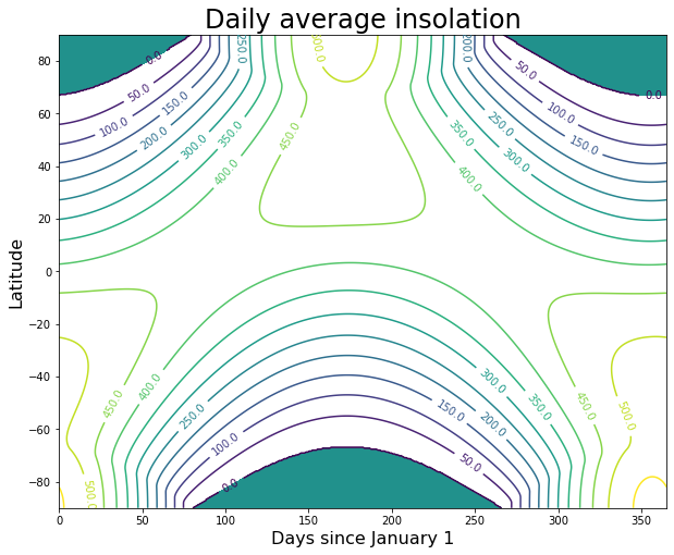
../_images/courseware_Insolation_8_0.png

Take the area-weighted global, annual average of Q…

[4]:

print(np.sum( np.mean( Q, axis=1 ) * np.cos( np.deg2rad(lat) ) ) / np.sum( np.cos( np.deg2rad( lat ) ) ))

341.38418448107586

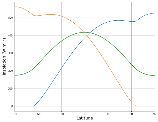
Also plot the zonally averaged insolation at a few different times of the year:

[5]:

summer_solstice = 170
winter_solstice = 353
ax = plt.figure( figsize=(10,8) ).add_subplot(111)
ax.plot( lat, Q[:,(summer_solstice, winter_solstice)] );
ax.plot( lat, np.mean(Q, axis=1), linewidth=2 )
ax.set_xbound(-90, 90)
ax.set_xticks( range(-90,100,30) )
ax.set_xlabel('Latitude', fontsize=16 );
ax.set_ylabel('Insolation (W m$^{-2}$)', fontsize=16 );
ax.grid()
plt.show()

../_images/courseware_Insolation_12_0.png

Past orbital parameters¶

The orbital.py code allows us to look up the orbital parameters for Earth over the last 5 million years.

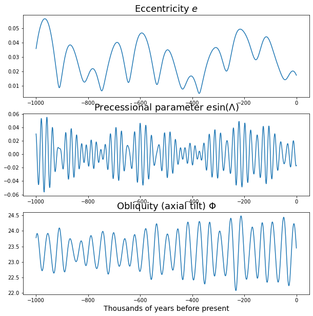
Make reference plots of the variation in the three orbital parameter over the last 1 million years

[6]:

from climlab.solar.orbital import OrbitalTable

kyears = np.arange( -1000., 1.)
#table = OrbitalTable()
orb = OrbitalTable.interp(kyear=kyears )
orb

Tokenization took: 2.07 ms
Type conversion took: 1.39 ms
Parser memory cleanup took: 0.01 ms

The xarray object orb now holds 1 million years worth of orbital data, total of 1001 data points for each element: eccentricity ecc, obliquity angle obliquity, and solar longitude of perihelion long_peri.

[7]:

fig = plt.figure( figsize = (10,10) )
ax1 = fig.add_subplot(3,1,1)
ax1.plot( kyears, orb['ecc'] )
ax1.set_title('Eccentricity $e$', fontsize=18 )
ax2 = fig.add_subplot(3,1,2)
ax2.plot( kyears, orb['ecc'] * np.sin( np.deg2rad( orb['long_peri'] ) ) )
ax2.set_title('Precessional parameter $e \sin(\Lambda)$', fontsize=18 )
ax3 = fig.add_subplot(3,1,3)
ax3.plot( kyears, orb['obliquity'] )
ax3.set_title('Obliquity (axial tilt) $\Phi$', fontsize=18 )
ax3.set_xlabel( 'Thousands of years before present', fontsize=14 )
plt.show()

../_images/courseware_Insolation_18_0.png

Annual mean insolation¶

Create a large array of insolation over the whole globe, whole year, and for every set of orbital parameters.

[8]:

lat = np.linspace(-90, 90, 181)
days = np.linspace(1.,50.)/50 * const.days_per_year
Q = daily_insolation(lat, days, orb)
print(Q.shape)

(181, 50, 1001)

[9]:

Qann = np.mean(Q, axis=1)  # time average over the year
print(Qann.shape)
Qglobal = np.empty_like( kyears )
for n in range( kyears.size ):   # global area-weighted average
    Qglobal[n] = np.sum( Qann[:,n] * np.cos( np.deg2rad(lat) ) ) / np.sum( np.cos( np.deg2rad(lat) ) )
print(Qglobal.shape)

(181, 1001)
(1001,)

We are going to create a figure showing past time variations in three quantities:

Global, annual mean insolation
Annual mean insolation at high northern latitudes
Summer solstice insolation at high northern latitudes

[10]:

fig = plt.figure( figsize = (10,14) )

ax1 = fig.add_subplot(3,1,1)
ax1.plot( kyears, Qglobal )
ax1.set_title('Global, annual mean insolation', fontsize=18 )
ax1.ticklabel_format( useOffset=False )

ax2 = fig.add_subplot(3,1,2)
ax2.plot( kyears, Qann[160,:] )
ax2.set_title('Annual mean insolation at 70N', fontsize=18 )

ax3 = fig.add_subplot(3,1,3)
ax3.plot( kyears, Q[160,23,:] )
ax3.set_title('Summer solstice insolation at 70N', fontsize=18 )

plt.show()

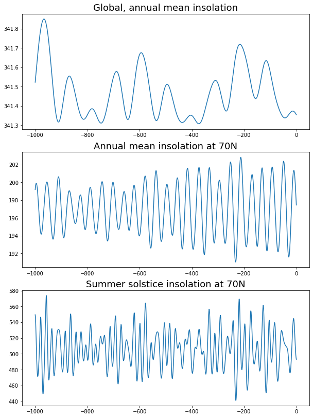
../_images/courseware_Insolation_24_0.png

And comparing with the plots of orbital variations above, we see that

Global annual mean insolation variations on with eccentricity (slow), and the variations are very small!
Annual mean insolation varies with obliquity (medium). Annual mean insolation does NOT depend on precession!
Summer solstice insolation at high northern latitudes is affected by both precession and obliquity. The variations are large.

Insolation changes between the Last Glacial Maximum and the end of the last ice age¶

Last Glacial Maximum or “LGM” occurred around 23,000 years before present, when the ice sheets were at their greatest extent. By 10,000 years ago, the ice sheets were mostly gone and the last ice age was over. Let’s plot the changes in the seasonal distribution of insolation from 23 kyrs to 10 kyrs.

[11]:

orb_0 = OrbitalTable.interp(kyear=0)  # present-day orbital parameters
orb_10 = OrbitalTable.interp(kyear=-10)  # orbital parameters for 10 kyrs before present
orb_23 = OrbitalTable.interp(kyear=-23)   # 23 kyrs before present
Q_0 = daily_insolation( lat, days, orb_0 )
Q_10 = daily_insolation( lat, days, orb_10 )   # insolation arrays for each of the three sets of orbital parameters
Q_23 = daily_insolation( lat, days, orb_23 )

[12]:

fig = plt.figure( figsize=(20,8) )

ax1 = fig.add_subplot(1,2,1)
Qdiff = Q_10 - Q_23
CS1 = ax1.contour( days, lat, Qdiff, levels = np.arange(-100., 100., 10.) )
ax1.clabel(CS1, CS1.levels, inline=True, fmt='%r', fontsize=10)
ax1.contour( days, lat, Qdiff, levels = [0.], colors = 'k' )
ax1.set_xlabel('Days since January 1', fontsize=16 )
ax1.set_ylabel('Latitude', fontsize=16 )
ax1.set_title('Insolation differences: 10 kyrs - 23 kyrs', fontsize=24 )

ax2 = fig.add_subplot(1,2,2)
ax2.plot( np.mean( Qdiff, axis=1 ), lat )
ax2.set_xlabel('W m$^{-2}$', fontsize=16 )
ax2.set_ylabel( 'Latitude', fontsize=16 )
ax2.set_title(' Annual mean differences', fontsize=24 )
ax2.set_ylim((-90,90))
ax2.grid()

plt.show()

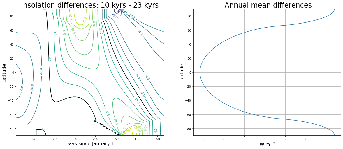
../_images/courseware_Insolation_29_0.png

The annual mean plot shows a classic obliquity signal: at 10 kyrs, the axis close to its maximum tilt, around 24.2º. At 23 kyrs, the tilt was much weaker, only about 22.7º. In the annual mean, a stronger tilt means more sunlight to the poles and less to the equator. This is very helpful if you are trying to melt an ice sheet.

Finally, take the area-weighted global average of the difference:

[13]:

print(np.average(np.mean(Qdiff,axis=1), weights=np.cos(np.deg2rad(lat))))

0.0065104307832676315

This confirms that the difference is tiny (and due to very small changes in the eccentricity). Ice ages are driven by seasonal and latitudinal redistributions of solar energy, NOT by changes in the total global amount of solar energy!

Table of Contents

This Page

Distribution of insolation¶

Present-day orbital parameters¶

Past orbital parameters¶

Annual mean insolation¶

Insolation changes between the Last Glacial Maximum and the end of the last ice age¶