BudykoTransport

class climlab.dynamics.budyko_transport.BudykoTransport(b=3.81, **kwargs)

Bases: EnergyBudget

calculates the 1 dimensional heat transport as the difference between the local temperature and the global mean temperature.

Parameters:

b (float) – Budyko transport parameter in units of \(\textrm{W} / \left( \textrm{m}^2 \ ^{\circ} \textrm{C} \right)\) [default value: 3.81]

As BudykoTransport is a Process it needs a state do be defined on. See example for details.

Computation Details:

In a global Energy Balance Model

\[C \frac{dT}{dt} = R\downarrow - R\uparrow - H\]

with model state \(T\), the energy transport term \(H\) can be described as

\[H = b [T - \bar{T}]\]

where \(T\) is a vector of the model temperature and \(\bar{T}\) describes the mean value of \(T\).

For further information see Budyko [1969].

Example:

Budyko Transport as a standalone process:

import climlab
from climlab.dynamics.budyko_transport import BudykoTransport
from climlab import domain
from climlab.domain import field
from climlab.utils.legendre import P2
import numpy as np
import matplotlib.pyplot as plt

# create domain
sfc = domain.zonal_mean_surface(num_lat = 36)

lat = sfc.lat.points
lat_rad = np.deg2rad(lat)

# define initial temperature distribution
T0 = 15.
T2 = -20.
Ts = field.Field(T0 + T2 * P2(np.sin(lat_rad)), domain=sfc)

# create BudykoTransport process
budyko_transp = BudykoTransport(state=Ts)

### Integrate & Plot ###

fig = plt.figure( figsize=(6,4))
ax = fig.add_subplot(111)

for i in np.arange(0,3,1):  
    ax.plot(lat, budyko_transp.default, label='day %s' % (i*40))
    budyko_transp.integrate_days(40.)

ax.set_title('Standalone Budyko Transport')
ax.set_xlabel('latitude')
ax.set_xticks([-90,-60,-30,0,30,60,90])
ax.set_ylabel('temperature ($^{\circ}$C)')
ax.legend(loc='best')
plt.show()

(Source code, png, hires.png, pdf)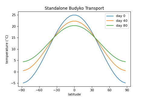

Attributes:

b

the budyko transport parameter in unit

current_time

depth

Depth at grid centers (m)

depth_bounds

Depth at grid interfaces (m)

diagnostics

Dictionary access to all diagnostic variables

elapsed_time

input

Dictionary access to all input variables

lat

Latitude of grid centers (degrees North)

lat_bounds

Latitude of grid interfaces (degrees North)

lev

Pressure levels at grid centers (hPa or mb)

lev_bounds

Pressure levels at grid interfaces (hPa or mb)

lon

Longitude of grid centers (degrees)

lon_bounds

Longitude of grid interfaces (degrees)

timestep

The amount of time over which step_forward() is integrating in unit seconds.

timestep_in_seconds

Return a float value representing the timestep in units of seconds

Methods

add_diagnostic(name[, value])	Create a new diagnostic variable called name for this process and initialize it with the given value.
add_input(name[, value])	Create a new input variable called name for this process and initialize it with the given value.
add_subprocess(name, proc[, verbose])	Adds a single subprocess to this process.
add_subprocesses(procdict)	Adds a dictionary of subproceses to this process.
compute()	Computes the tendencies for all state variables given current state and specified input.
compute_diagnostics([num_iter])	Compute all tendencies and diagnostics, but don't update model state.
declare_diagnostics(diaglist)	Add the variable names in inputlist to the list of diagnostics.
declare_input(inputlist)	Add the variable names in inputlist to the list of necessary inputs.
integrate_converge([crit, verbose])	Integrates the model until model states are converging.
integrate_days([days, verbose])	Integrates the model forward for a specified number of days.
integrate_years([years, verbose])	Integrates the model by a given number of years.
remove_diagnostic(name)	Removes a diagnostic from the process.diagnostic dictionary and also delete the associated process attribute.
remove_subprocess(name[, verbose])	Removes a single subprocess from this process.
set_state(name, value)	Sets the variable name to a new state value.
step_forward()	Updates state variables with computed tendencies.
to_xarray([diagnostics, timeave])	Convert process variables to xarray.Dataset format.

property b

the budyko transport parameter in unit \(\frac{\textrm{W}}{\textrm{m}^2 \textrm{K}}\)

Getter:

returns the budyko transport parameter

Setter:

sets the budyko transport parameter

Type:

float